My question is basically from SeaDAS, so you can only see my SeaDAS configuration and the questions below. DINEOF is only for interpolation and therefore Figure 3.
I am trying to find a good configuration for a multivariate interpolation of SST and Chlorophyll-a in a group of islands in the South East Pacific. It is called the Juan Fernández Archipelago. I downloaded 1km L2 images of Modis-Aqua from the OceanColorWeb. The first challenge was to process them with SeaDAS to convert them to L3m format. As I read in the forum, the problem of MODIS is that it is nominally 1km at nadir, but it is not like that during all the scan, so you should work with a lower resolution. So I tried two configurations of Seadas, both with L2bin + L3mapgen: Working with resolution of 2km (170x275) and 1km (340x551) with the parameter "fudge" = 2 and 10. However, there is not much information about the consequences of use a very large number of "fudge" and in the forums I have seen it used in a range of 0 to 2 (but you can put any number: 1.5, 6, 10, etc.). As it is a very remote Island, there are not many data with which to compare, so I tried to make my images look like Figure 2 and 3 (attached) of the following paper, where they also use the same images and DINEOF:
Andrade, I., Sangrà, P., Hormazabal, S., & Correa-Ramirez, M. (2014). Island mass effect in the Juan Fernandez Archipelago (33 S), southeastern Pacific. Deep Sea Research Part I: Oceanographic Research Papers, 84, 86-99.
My configuration of SeaDAS is as follows (I will show only that of Chlorophyll-a):
For l2bin:
resolve = "2" # and then "1"
suite = "CHL"
flaguse = "ATMFAIL, LAND, HILT, HISATZEN, STRAYLIGHT, CLDICE, COCCOLITH, LOWLW, CHLWARN, CHLFAIL, NAVWARN, MAXAERITER, ATMWARN, HISOLZEN, NAVFAIL, FILTER, HIGLINT"
l3bprod = "chlor_a, chl_ocx"
prodtype = "regional" # if there is more than one image per day or "day" if not.
qual_max = "2"
oformat = "2"
night = "0"
average = "standard"
verbose = "1"
minobs = "0"
deflate = "4"
For l3mapgen
product = "chlor_a"
projection = "smi"
resolution = "2km" # and then "1km"
interp = "area"
north = "- 31.99"
south = "- 35.54"
east = "- 76.91"
west = "- 82.65"
oformat = "2"
deflate = "4"
product_rgb = "rhos_645, rhos_555, rhos_469"
fudge = "1.0" #and then 2 or 10
threshold = "0"
apply_pal = "1"
use_quality = "no"
use_rgb = "no"
suite = "CHL"
oformat2 = "png"
trimNSEW = "yes"
quiet = "false"
mask_land = "no"
land = "$ OCDATAROOT / common / landmask_GMT15ARC.nc"
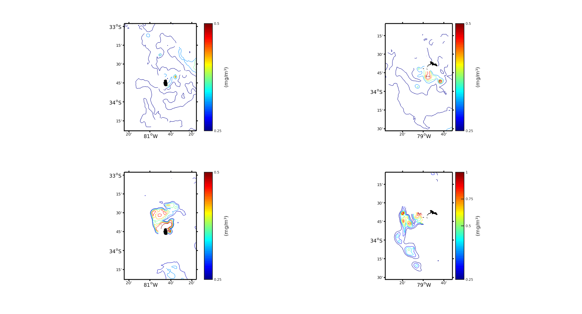
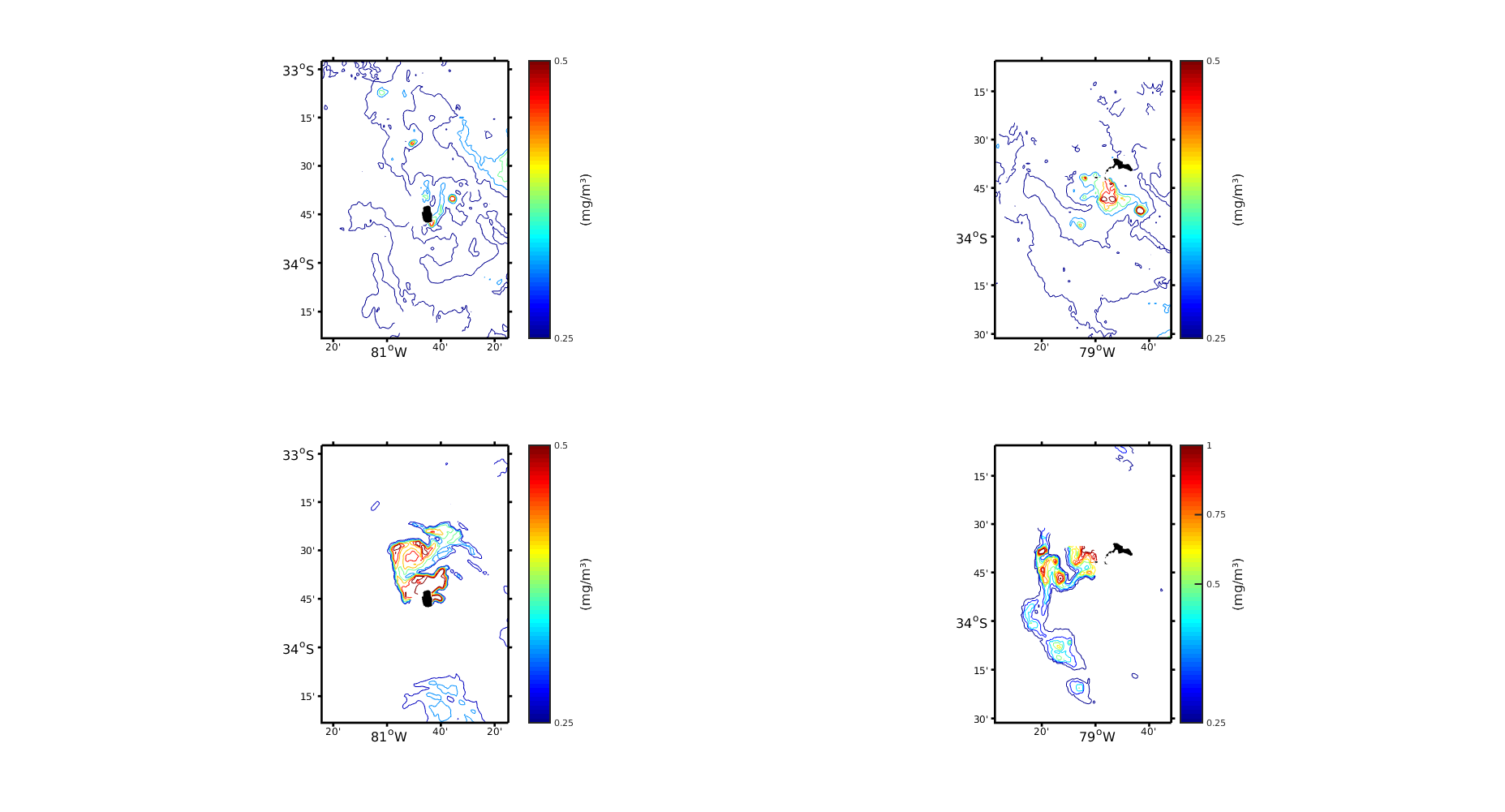
In the figures attached (Figure 2), it is clear that the 2km version looks much smoother and less noisy. The difference between increasing the fudge for the 1km images is that more structures appear and the contours of the plot are "completed". Now, in comparison with Figure 2 of Andrade et al., 2014 there is a kind of similarity between the figures. However, it seems that in Andrade et al., 2014 they are less "conservative" or more "flexible" since they have much more data in each scene.
Then, I applied DINEOF. Since this is not a DINEOF forum, I will only say that it was a multivariate interpolation of SST + Chlorophyll-a and that the only parameters that I changed were: numit = 6, nev = 12 and ncv = 21
1) And the resulting figures are attached (Figure 3). Now, looking at the different Figures 2 and 3 my question is: the difference I experience between my figures and those of the paper will be due to some problem in SeaDAS (which I believe) or to the configuration of DINEOF. In the paper they didn't occupied SeaDAS, that is one of the problems.
2) About the problem of the resolution. If I resigned and I have to work with 2 kilometers, is the correct thing to do l2bin with "resolve" = 1 and then l3mapgen with "resolution" = 2km, or "resolve" = 2 and "resolution" = 2km ?. And in the opposite case, if I want to "force" 1 kilometer, what happens if you put "resolve" = 2 and "resolution" = 1km ?. What happens is that I have seen contradictory answers in the forum.
Thank you!