Structure tensor

The structure tensor page is a general purpose description, tutorial and demonstration of the uses of this form.

Summary

Structure tensors are a matrix representation of partial derivative information. In the field of image processing and computer vision, it is typically used to represent the gradient or "edge" information. It also has a more powerful description of local patterns as opposed to the directional derivative through its coherence measure. It has several other advantages that are detailed in the structure tensor section of this tutorial. This information is designed specifically as either an introduction or refresher to structure tensors to those in the image processing field; however, it should also be useful to those from a more general math background who want to learn more about this matrix representation. To provide more detail than the typical tutorial, I have included the MATLAB source code both as inline with the text as well as in a comprehensive zip file at the end of this document.

Background

Gradient

 

Gradient information serves several purposes. It can relate the structure of objects in an image, identify features of interest for recognition/classification directly or provide the basis of further processing for various computer vision tasks. For example, "edges," noted by regions of high gradient magnitude, are central to the task of identifying defects in circuitry. A sample "edge-detected" image created using the 'Image Processing Toolbox' for MATLAB is shown where locations marked by white are those points that are indicative of high gradient magnitude, which can also be described as regions of high pixel contrast.

Directional derivative

File:DDoneArrow.jpg

File:StepDDorient.jpg

File:CoherenceCases.png

When representing gradient information derived from an image, there are several options from which to choose. One such choice is the directional derivative that provides a vector representation. Its magnitude reflects the maximum change in pixel values while the phase is directed along the orientation corresponding to the maximum change. These two components are calculated as per Equations (1) and (2) respectively:

File:DDmagEqn.png

File:DDphaseEqn.png

where ${\displaystyle I_{x}}$  denotes the partial derivative of image ${\displaystyle I}$  along the ${\displaystyle x}$ -axis. An example is shown against a horizontal step-edge image with the directional derivative overlaid with a red arrow.

The direction of the gradient in this case is based purely on the ordering of the pixel values. i.e. it points from black to white. If these colors were reversed, the gradient magnitude would remain the same; however, the direction would then be reversed such that it again pointed FROM the black TO the white region. In applications where the gradient is used to denote contours within the scene, such as object outlines, the polarity is of little use. Nevertheless, this orientation reveals the "normal" to the contour in question. "Orientation," in this context, implies PI-periodic behavior, as in the term "horizontal orientation." i.e. orientation ranges between ${\displaystyle [0,\pi )}$ . To reflect this periodicity, the directional derivative, when applied to the extraction of gradient-based structures, should also have an arrow pointed in the opposite direction.

Although the directional derivative is relatively computational inexpensive, it does possess a weakness. This is best illustrated with an example. Given an isotropic structure, where there is no preferred direction of gradient, the directional derivative formula results in a zero magnitude. An example of such an isotropic structure is a black circle on a white background. There is clearly gradient information; however, since there is no preferred phase, it zeros itself out.

There are several ways to calculate the partial derivatives of the image. For example, simple differencing between neighboring pixels one option, although the gradient will only be representative of a ${\displaystyle 2x1}$  region of interest. The 'Difference of Gaussians' (DoG) is a common technique that convolves a specialized mask to calculate the partial derivative value over a larger region of interest.

The same output is reached if the original input is a uniformly colored region. Again, the directional derivative magnitude is zero as there is no gradient information with which to calculate. What is needed is a representation capable of discerning between these two examples that properly reflects the presence of gradient information in the first case, but none in the second.

Structure tensors

Overview

A different method of representing gradient information is by using the "structure tensor." It also makes use of the ${\displaystyle I_{x}}$  and ${\displaystyle I_{y}}$  values, however, in a matrix form. The term tensor refers to a representation of an array of data. The "rank" of a tensor denotes the number of indices needed to describe it. For example, a scalar value ${\displaystyle x}$  is a single value, hence requires no indices. This means that a scalar is a tensor of rank zero. A vector ${\displaystyle {\vec {v}}}$ , often represented as ${\displaystyle v_{i}=\{v_{1},v_{2},..v_{n}\}}$  uses a single index, ${\displaystyle i}$ . This implies that a vector is a tensor of rank one. A two-dimensional matrix ${\displaystyle M_{ij}}$  is a tensor of rank two and so and so forth.

2D structure tensor

The structure tensor matrix (also referred to as the "second-moment matrix") is formed as:

File:STeqn2D.png

Eigen-decomposition is then applied to the structure tensor matrix ${\displaystyle S}$  to form the eigenvalues and eigenvectors ${\displaystyle (\lambda _{1},\lambda _{2})}$  and ${\displaystyle ({\vec {e}}_{1},{\vec {e}}_{2})}$  respectively. These new gradient features allow a more precise description of the local gradient characteristics. For example, ${\displaystyle {\vec {e}}_{1}}$ , is a unit vector directed normal to the gradient edge, while the ${\displaystyle {\vec {e}}_{2}}$  vector is tangent. The eigenvalues indicate the underlying certainty of the gradient structure along their associated eigenvector directions. As noted by several researchers, the "coherence" is obtained as a function of the eigen-values^{[1] [2] [3]}. This value is capable of distinguishing between the isotropic and uniform cases. The coherence is calculated as per the following equation:

File:CoherenceEqn.png

If a different method is used to obtain the partial derivative information, for example using Horn's approach where the average, absolute pixel difference is used, the coherence for the isotropic region is one while the uniform case is zero: opposite of the values obtained above. What is key is that no matter the partial derivative method used, the coherence, a feature of the structure tensor, is able to distinguish between the two cases.

Many corner detection and salient point ___location algorithms ^{[4] [5] [6] [7]} make use of the eigenvalues that are derived from the structure tensor to quantify the certainty in the measurements ^[8]

There are other advantages to using the structure tensor representation as well. For example, local shifting of edge locations in minimized when applying a Gaussian smoothing operator element-by-element to the structure tensor ^[9]. Furthermore, the cancellations of opposing gradient polarity directions are prevented when structure tensors are summed ^[10].

For scale-space properties of the structure tensor (or second-moment matrix) when using a Gaussian window function for integration, please refer to ^[11][12]. For the application of the structure tensor to non-linear fingerprint enhancement, please see ^[13].

3D structure tensors

Overview

 

Elliptical representation of structure tensor

This form of gradient representation serves especially well in inferring structure from sparse and noisy data [Medioni et al. 2000]. The structure tensor is also applicable to higher dimensional data. For example, given three-dimensional data, such as that from a spatio-temporal volume ${\displaystyle (x,y,time)}$  or medical imaging input ${\displaystyle (x,y,z)}$ , the structure tensor is represented as follows:

File:STeqn3D.png

The eigen-decomposition of the tensor of rank two results in ${\displaystyle (\lambda _{1},\lambda _{2},\lambda _{3})}$  and ${\displaystyle ({\vec {e}}_{1},{\vec {e}}_{2},{\vec {e}}_{3})}$  for the eigenvalues and eigenvectors respectively. The interpretation of these components can be visualized as 3D ellipses where the radii are equal to the eigenvalues in descending order and directed along their corresponding eigenvectors.

3d structure types

The differences between the eigenvalues indicate underlying structure as well. For example, if the value of ${\displaystyle (\lambda _{1}-\lambda _{2})>>0}$ , this depicts a "surfel" surface element, where ${\displaystyle {\vec {e}}_{1}}$  is the normal to the surface^[9].

•  
  A local curve element, "curvel," is identified as ${\displaystyle (\lambda _{2}-\lambda _{3})>>0}$  where ${\displaystyle {\vec {e}}_{3}}$  is tangent to the curve.
•  
  If ${\displaystyle \lambda _{3}>>0}$  then there is presence of an isotropic behavior, similar to a spherical structure or uniform region.
•  

3D results

Applied against actual data

•  
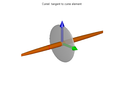
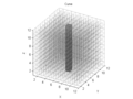
  Step plane case
•  
  Associated structure tensor in elliptical form
•  
  Curve case
•  
  Associated structure tensor in elliptical form
•  
  Sphere case
•  
  Associated structure tensor in elliptical form

Tensor addition

File:TensorAddition.png

Tensor addition of sphere and step-edge case

Another desirable property of the structure tensor form is that the tensor addition equates itself to the adding of the elliptical forms. For example, if the structure tensors for the sphere case and step-edge case are added, the resulting structure tensor is an elongated ellipsed along the direction of the step-edge case.

Applications

Although structure tensors are applicable to many ND domains, it is in the image processing / computer vision domains that is of considerable interest. Using gradient-based structure tensors, local patterns of contours and surfaces may be inferred through a diffusion process ^[14]. Diffusion aids to enforce local structural estimates that serve such applications as defect detection in lumber, occlusion detection in image sequences and aid in biometric identification of fingerprints ^[15].

References

1. B. Jahne (1993). Spatio-Temporal Image Processing: Theory and Scientific Applications. Vol. 751. Berlin: Springer-Verlag.
2. G. Medioni, M. Lee and C. Tang (2000). A Computational Framework for Feature Extraction and Segmentation. Elsevier Science. {{cite book}}: Unknown parameter |month= ignored (help); line feed character in |title= at position 49 (help)
3. D. Tschumperle and Deriche (2002). "Diffusion PDE's on Vector-Valued Images": 16–25. {{cite journal}}: Cite journal requires |journal= (help); Unknown parameter |booktitle= ignored (help); Unknown parameter |month= ignored (help)
4. W. Forstner (1986). "A Feature Based Correspondence Algorithm for Image Processing". 26: 150–166. {{cite journal}}: Cite journal requires |journal= (help); Unknown parameter |booktitle= ignored (help)
5. C. Harris and M. Stephens (1988). "A Combined Corner and Edge Detector". Proc. of the 4th ALVEY Vision Conference. pp. 147–151. {{cite conference}}: Unknown parameter |booktitle= ignored (|book-title= suggested) (help)
6. K. Rohr (1997). "On 3D Differential Operators for Detecting Point Landmarks". 15 (3): 219–233. {{cite journal}}: Cite journal requires |journal= (help); Unknown parameter |booktitle= ignored (help)
7. B. Triggs (2004). "Detecting Keypoints with Stable Position, Orientation, and Scale under Illumination Changes". Proc. European Conference on Computer Vision. Vol. 4. pp. 100–113. {{cite conference}}: Unknown parameter |booktitle= ignored (|book-title= suggested) (help)
8. C. Kenney, M. Zuliani and B. Manjunath, (2005). "An Axiomatic Approach to Corner Detection". Proc. IEEE Computer Vision and Pattern Recognition. pp. 191–197. {{cite conference}}: Unknown parameter |booktitle= ignored (|book-title= suggested) (help)
9. M. Nicolescu and G. Medioni (2003). "Motion Segmentation with Accurate Boundaries — A Tensor Voting Approach". Proc. IEEE Computer Vision and Pattern Recognition. Vol. 1. pp. pp.382–389. {{cite conference}}: |pages= has extra text (help); Unknown parameter |booktitle= ignored (|book-title= suggested) (help)
10. T. Brox, J. Weickert, B. Burgeth and P. Mrazek (2004). "Nonlinear Structure Tensors" (113): 1–32. {{cite journal}}: Cite journal requires |journal= (help); Unknown parameter |booktitle= ignored (help)
11. T. Lindeberg: Scale-Space Theory in Computer Vision, Kluwer Academic Publishers, Dordrecht, Netherlands, 1994.
12. [http://www.nada.kth.se/cvap/abstracts/cvap117.html J. Garding and T. Lindeberg: "Direct computation of shape cues using scale-adapted spatial derivative operators, International Journal of Computer Vision, vol 17(2), pp. 163--191, 1996.
13. A. Almansa and T. Lindeberg, ``Enhancement of fingerprint images using shape-adaptated scale-space operators, IEEE Transactions on Image Processing, volume 9, number 12, pp 2027-2042, 2000
14. S. Arseneau and J. Cooperstock (2006). "An Asymmetrical Diffusion Framework for Junction Analysis". British Machine Vision Conference. Vol. 2. pp. 689–698. {{cite conference}}: Unknown parameter |booktitle= ignored (|book-title= suggested) (help); Unknown parameter |month= ignored (help); line feed character in |title= at position 49 (help)
15. S. Arseneau, and J. Cooperstock (2006). "An Improved Representation of Junctions through Asymmetric Tensor Diffusion". International Symposium on Visual Computing. {{cite conference}}: Unknown parameter |booktitle= ignored (|book-title= suggested) (help); Unknown parameter |month= ignored (help)

See Also

• Tensor
• Directional derivative
• Gaussian
• Corner detection
• Edge detection

Resources

• Download MATLAB Source
• Structure Tensor Tutorial (Original)