Utente:Etrusko25/Sandbox 3

La rete alimentare pelagica, che mostra il ruolo centrale dei microrganismi marini nel modo in cui l'oceano importa nutrienti dall'atmosfera e li esporta nuovamente verso l'atmosfera e il fondo oceanico.

La rete alimentare marina è la rete alimentare negli ambienti marini e oceanici. Alla base della rete alimentare oceanica ci sono alghe unicellulari e altri organismi fotosintetici noti come fitoplancton. Il secondo livello trofico (consumatori primari) è occupato dallo zooplancton, che si nutre del fitoplancton. I consumatori di ordine superiore completano la rete. Nel tempo è cresciuta la consapevolezza riguardo ai microrganismi marini.

L'habitat determina variazioni nelle reti alimentari. Le reti di interazioni trofiche possono anche fornire molte informazioni sul funzionamento degli ecosistemi marini.

Rispetto agli ambienti terrestri, gli ambienti marini presentano piramidi di biomassa invertite alla base. In particolare, la biomassa dei consumatori (copepodi, krill, gamberetti, pesci foraggio) è maggiore della biomassa dei produttori primari. Ciò accade perché i produttori primari dell'oceano sono minuscoli organismi del fitoplancton che crescono e si riproducono rapidamente, quindi una piccola massa può avere un rapido tasso di produzione primaria. Al contrario, molti importanti produttori primari terrestri, come le foreste mature, crescono e si riproducono lentamente, quindi è necessaria una massa molto più grande per ottenere lo stesso tasso di produzione primaria. A causa di questa inversione, è lo zooplancton a costituire la maggior parte della biomassa negli ambienti marini.

Catena trofica e livelli trofici

  Voci principali: Catena alimentare, Livello trofico.

Le reti trofiche sono costituite da catene alimentari. Tutte le forme di vita presenti nel mare hanno il potenziale per diventare cibo per altre forme di vita. Nell'oceano, una catena alimentare inizia tipicamente con l'energia del sole che alimenta il fitoplancton e segue un iter simile al seguente:

fitoplancton → zooplancton erbivoro → zooplancton carnivoro → filtratore → vertebrato predatore

Il fitoplancton non ha bisogno di altri organismi per nutrirsi, poiché è in grado di produrre il proprio alimento direttamente dal carbonio inorganico, utilizzando la luce solare come fonte di energia. Questo processo è chiamato fotosintesi e porta il fitoplancton a convertire il carbonio presente in natura in protoplasma. Per questo motivo, il fitoplancton è considerato il produttore primario alla base della catena alimentare marina. Poiché si trova al primo livello, si dice che abbia un livello trofico pari a 1. Il fitoplancton viene poi consumato al livello trofico successivo nella catena alimentare da animali microscopici chiamati zooplancton.

Lo zooplancton costituisce il secondo livello trofico nella catena alimentare e comprende organismi microscopici unicellulari come i protozoi, piccoli crostacei come i copepodi e il krill e larve di pesci, cefalopodi, aragoste e granchi. Gli organismi a questo livello possono essere considerati come consumatori primari.

A loro volta, gli zooplanctonti erbivori più piccoli vengono consumati dagli zooplanctonti carnivori più grandi, come i protozoi predatori più grandi e il krill, e dai pesci foraggio, che sono piccoli pesci che vivono in banchi e si nutrono filtrando l'acqua. Si tratta del terzo livello trofico nella catena alimentare.

 

Una rete alimentare è un insieme di catene alimentari e, in quanto tale, può essere rappresentata graficamente e analizzata utilizzando le tecniche della teoria delle reti.^[1][2]

 

Rete alimentare tipica delle foche grigie nel mar Baltico, che comprende diverse catene alimentari marine caratteristiche.^[3]

Il quarto livello trofico è costituito da pesci predatori, mammiferi marini e uccelli marini che si nutrono di pesci foraggio. Ne sono un esempio il pesce spada, le foche e le sule.

I predatori apicali, come le orche, che possono nutrirsi di foche, e gli squali mako, che possono nutrirsi di pesci spada, costituiscono il quinto livello trofico. Le balene possono nutrirsi direttamente di zooplancton e krill, dando vita a una catena alimentare con solo tre o quattro livelli trofici.

In pratica, i livelli trofici non sono solitamente numeri interi semplici perché la stessa specie consumatrice spesso si nutre attraverso più di un livello.^[4][5] Ad esempio, un grande vertebrato marino può nutrirsi di pesci predatori più piccoli, ma anche di organismi filtratori; la pastinaca si nutre di crostacei, mentre lo squalo martello si nutre sia di crostacei che di pastinache. Gli animali possono anche nutrirsi l'uno dell'altro; il merluzzo mangia merluzzi più piccoli e gamberi, mentre i gamberi si nutrono di larve di merluzzo. Le abitudini alimentari di un animale giovane e, di conseguenza, il suo livello trofico, possono cambiare con la crescita.

Il biologo della pesca Daniel Pauly assegna i valori dei livelli trofici come segue: uno ai produttori primari e al detrito, due agli erbivori e ai detritivori (consumatori primari), tre ai consumatori secondari e così via. La definizione del livello trofico(TL) per qualsiasi specie consumatrice è^[6]

${\displaystyle TL_{i}=1+\sum _{j}(TL_{j}\cdot DC_{ij}),}$ 

dove ${\displaystyle TL_{j}}$  è il livello trofico frazionario della preda j, e ${\displaystyle DC_{ij}}$  rappresenta la frazione di j nella dieta di i. Nel caso degli ecosistemi marini, il livello trofico della maggior parte dei pesci e degli altri consumatori marini assume valori compresi tra 2,0 e 5,0. Il valore superiore, 5,0, è insolito, anche per i pesci di grandi dimensioni,^[7] anche se si riscontra nei predatori apicali dei mammiferi marini come gli orsi polari e le orche.^[8] Per fare un confronto, gli esseri umani hanno un livello trofico medio di circa 2,21, più o meno lo stesso di un maiale o di un'acciuga.^[9][10]

Per taxon

Produttori primari

 

Concentrazione di clorofilla sulla superficie oceanica nell'ottobre 2019. La concentrazione di clorofilla può essere utilizzata come indicatore della quantità di fitoplancton presente. Pertanto su questa mappa globale il verde indica dove è presente una maggior quantità di fitoplancton, mentre il blu indica dove ne è presente una quantità ridotta. – NASA Earth Observatory 2019.^[11]

  Lo stesso argomento in dettaglio: Produzione primaria marina.

Alla base della catena alimentare oceanica ci sono alghe unicellulari e altri organismi simili alle piante noti come fitoplancton. Il fitoplancton è un gruppo di autotrofi microscopici appartenenti a gruppi tassonomici classificati in base alla morfologia, alle dimensioni e al tipo di pigmento. Il fitoplancton marino vive principalmente nelle acque superficiali illuminate dal sole come fotoautotrofi e necessita di nutrienti come azoto e fosforo, oltre che della luce solare per fissare il carbonio e produrre ossigeno. Tuttavia, alcuni fitoplanctonti marini vivono in profondità, spesso vicino alle sorgenti idrotermali, come chemoautotrofi che utilizzano fonti di elettroni inorganici come idrogeno solforato, ferro ferroso e ammoniaca.^[12]

Non è possibile comprendere un ecosistema senza conoscere il modo in cui la sua rete alimentare determina il flusso di materiali ed energia. Il fitoplancton produce biomassa in modo autotrofico convertendo i composti inorganici in composti organici. In questo modo, il fitoplancton funge da base della rete alimentare marina, sostenendo tutte le altre forme di vita nell'oceano. Il secondo processo centrale nella rete alimentare marina è il ciclo microbico. Questo ciclo degrada i batteri e gli archaea marini, rimineralizza la materia organica e inorganica e ricicla i prodotti all'interno della rete alimentare pelagica o depositandoli come sedimenti marini sul fondale. ^[13]

Il fitoplancton marino costituisce la base della catena alimentare marina e rappresenta circa la metà della fissazione globale di carbonio e della produzione di ossigeno attraverso la fotosintesi.^[14] ed è un anello fondamentale nel ciclo globale del carbonio.^[15] Come le piante sulla terraferma, il fitoplancton utilizza la clorofilla e altri pigmenti fotosintetici per svolgere la fotosintesi clorofilliana, assorbendo l'anidride carbonica atmosferica per produrre zuccheri da utilizzare come carburante metabolico. La clorofilla presente nell'acqua modifica il modo in cui l'acqua riflette e assorbe la luce solare, consentendo agli scienziati di mappare la quantità e la posizione del fitoplancton. Queste misurazioni forniscono agli scienziati preziose informazioni sullo stato di salute dell'ambiente oceanico e li aiutano a studiare il ciclo del carbonio oceanico.^[11]

Se gli organismi del fitoplancton muoiono prima di essere mangiat1, scendono attraverso la zona eufotica come parte della neve marina e si depositano nelle profondità oceaniche. In questo modo, il fitoplancton sequestra circa 2 miliardi di tonnellate di anidride carbonica nell'oceano ogni anno, trasformando l'oceano in un serbatoio di anidride carbonica che contiene circa il 90% di tutto il carbonio sequestrato.^[16] L'oceano produce circa la metà dell'ossigeno globale e immagazzina 50 volte più anidride carbonica rispetto all'atmosfera.^[17]

 

Prochlorococcus, un importante batterio che produce molto dell'ossigeno mondiale

Nel fitoplancton ci sono membri di un phylum di batteri chiamato cianobatteri. I cianobatteri marini includono gli organismi fotosintetici più piccoli conosciuti. Il più piccolo di tutti, Prochlorococcus, ha un diametro di soli 0,5-0,8 micrometri.^[18] In termini di numero di individui, Prochlorococcus è probabilmente la specie più abbondante sulla Terra: un solo millilitro di acqua marina superficiale può contenere 100.000 cellule o più. Si stima che in tutto il mondo esistano diversi ottilioni (10²⁷) di individui. Prochlorococcus è onnipresente tra i 40°N e i 40°S e domina nelle regioni oligotrofiche (povere di nutrienti) degli oceani.^[19] Questo batterio contribuisce per circa il 20% all'ossigeno presente nell'atmosfera terrestre.^[20]

• Il fitoplancton costituisce la base della catena alimentare marina
•  
  Fitoplancton
•  
  Dinoflagellato
•  
  Diatomee

Negli oceani la maggior parte della produzione primaria è svolta dalle alghe. Ciò è in contrasto con la terraferma, dove la maggior parte della produzione primaria è svolta dalle piante vascolari. Le alghe vanno dalle singole cellule galleggianti alle grandi alghe marine sessili, mentre le piante vascolari sono rappresentate nell'oceano da gruppi come le fanerogame marine e le mangrovie. I produttori più grandi, come le alghe marine e le fanerogame marine, sono per lo più confinati nella zona litorale e nelle acque poco profonde, dove si attaccano al substrato nell'ambito della zona eufotica. La maggior parte della produzione primaria da alghe è comunque svolta dal fitoplancton.

Pertanto, negli ambienti oceanici, il primo livello trofico è occupato principalmente dal fitoplancton, organismi microscopici, perlopiù alghe unicellulari, che fluttuano nel mare. La maggior parte del fitoplancton è troppo piccola per essere vista singolarmente ad occhio nudo. Quando è presente in quantità sufficientemente elevate, può apparire come una colorazione (spesso verde) dell'acqua. Poiché aumenta la propria biomassa principalmente attraverso la fotosintesi, vive nello strato superficiale illuminato dal sole del mare o zona eufotica.

I gruppi più importanti di fitoplancton includono le diatomee e i dinoflagellati. Le diatomee sono particolarmente importanti negli oceani, dove secondo alcune stime contribuiscono fino al 45% della produzione primaria totale dell'oceano^[21] Le diatomee sono solitamente microscopiche, anche se alcune specie possono raggiungere i 2 millimetri di lunghezza.

Consumatori primari

 

I ciliati oligotrichi sono considerati i più importanti erbivori oceanici

Il secondo livello trofico (consumatori primari) è occupato dallo zooplancton, che si nutre del fitoplancton. Insieme al fitoplancton, costituisce la base della piramide alimentare che sostiene la maggior parte delle grandi zone di pesca del mondo. Molti organismi dello zooplancton sono minuscoli animali che si trovano insieme al fitoplancton nelle acque superficiali oceaniche e comprendono piccoli crostacei, larve di pesci e avannotti. La maggior parte dello zooplancton è costituita da filtratori che utilizzano le appendici per filtrare il fitoplancton presente nell'acqua. Alcuni zooplanctonti di dimensioni maggiori si nutrono anche di zooplancton di minori dimensioni. Alcuni zooplanctonti possono spostarsi brevemente per sfuggire ai predatori, ma non sono in grado di nuotare. Come il fitoplancton, fluttuano seguendo le correnti, le maree e i venti. Lo zooplancton può riprodursi rapidamente e, in condizioni favorevoli, la sua popolazione può aumentare fino al trenta per cento al giorno. Molti hanno vita breve e raggiungono rapidamente la maturità.

Gli Oligotrichia sono un gruppo di ciliati che presentano ciglia orali sporgenti disposte come un collare. Sono molto comuni nelle comunità di plancton marino, dove solitamente si trovano in concentrazioni di circa uno per millilitro. Sono i più importanti consumatori primari marini, il primo anello della catena alimentare.^[22]

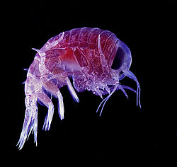
Altri gruppi particolarmente importanti di zooplancton sono i copepodi e il krill. I copepodi sono un gruppo di piccoli crostacei che vivono sia negli oceani che negli habitat d'acqua dolce. Sono la principale fonte di proteine in ambiente marino,^[23] e costituiscono una preda importante per i pesci foraggio. Il krill è la seconda fonte di proteine più importante. Il krill è costituito da zooplanctonti predatori di dimensioni relativamente grandi che si nutre di zooplancton di taglia inferiore. Ciò significa che appartiene al terzo livello trofico, quello dei consumatori secondari, insieme ai pesci foraggio.

• Lo zooplancton costituisce il secondo livello della catena alimentare oceanica
•  
  Polichete planctonico (Tomopteris)
•  
  Anfipode Hyperiidea
•  
  Giovanile di calamaro della famiglia Cranchiidae

 

Le meduse sono facili da catturare e digerire e potrebbero essere una fonte di cibo più importante di quanto si sia pensato finora.^[24]

Il fitoplancton e lo zooplancton insieme costituiscono la maggior parte del plancton presente nel mare. Il termine plancton indica qualsiasi piccolo organismo che galleggia nel mare (greco planktos = vagabondo o vagante). Per definizione, gli organismi classificati come plancton non sono in grado di nuotare contro le correnti oceaniche; non possono resistere alla corrente ambientale e controllare la loro posizione. Negli ambienti oceanici, i primi due livelli trofici sono occupati principalmente dal plancton. Il plancton può essere suddiviso in produttori e consumatori. I produttori sono il fitoplancton (dal greco phyton = pianta) e i consumatori, che si nutrono del fitoplancton, sono lo zooplancton (dal greco zoon = animale).

Le meduse nuotano lentamente e la maggior parte delle specie fa parte del plancton. Tradizionalmente, le meduse sono state considerate come un vicolo cieco trofico. Con un corpo costituito in gran parte da acqua, erano generalmente considerate come aventi un impatto limitato sugli ecosistemi marini, attirando l'attenzione di predatori specializzati come il pesce luna e la tartaruga liuto.^[25][24] Questa visione è stata recentemente messa in discussione. Le meduse e, più in generale, lo zooplancton gelatinoso, che comprende anche le salpe e gli ctenofori, sono molto diversificati, fragili, privi di parti dure, difficili da osservare e monitorare, soggetti a rapidi cambiamenti di popolazione e spesso vivono in luoghi scomodi, lontani dalla costa o nelle profondità dell'oceano. È difficile per gli studiosi individuare e analizzare le meduse nell'intestino dei predatori, poiché una volta ingerite si trasformano in poltiglia e vengono rapidamente digerite.^[25] Tuttavia, le meduse formano popolazioni abbondantissime ed è stato dimostrato che costituiscono una componente importante nella dieta dei tonni, marlin e pesci spada nonché di vari uccelli e invertebrati come polpi, cetrioli di mare, granchi e anfipodi.^[26][24] "Nonostante la loro bassa densità energetica, il contributo delle meduse al bilancio energetico dei predatori potrebbe essere molto maggiore di quanto si pensi, grazie alla rapida digestione, ai bassi costi di cattura, alla disponibilità e alla predazione selettiva dei componenti più ricchi di energia. Nutrirsi di meduse può rendere i predatori marini suscettibili all'ingestione di plastica."^[24]

Consumatori di ordine superiore

[[File:Schooling fish.jpg|thumb|upright=1.84|Pesci predatori (Siganus vulpinus) valutano le dimensioni dei pesci foraggio che nuotano in banchi

Invertebrati marini

Pesci

• Pesci foraggio: I pesci foraggio occupano una posizione centrale nella catena alimentare oceanica. Gli organismi di cui si nutrono si trovano a un livello trofico inferiore, mentre gli organismi che se ne cibano si trovano a un livello trofico superiore. I pesci foraggio occupano i livelli intermedi della catena alimentare, fungendo da preda principale per i pesci di livello superiore, gli uccelli marini e i mammiferi.
• Pesci predatori
• Pesci demersali

Altri vertebrati marini

Nel 2010, alcuni ricercatori hanno scoperto che le balene trasportano sostanze nutritive dalle profondità dell'oceano alla superficie utilizzando un processo che prende il nome inglese "whale pump" (pompa delle balene).^[27] Le balene si nutrono nelle parti profonde dell'oceano dove si trova il krill, ma tornano regolarmente in superficie per respirare. Lì le balene rilasciano le loro feci ricche di azoto e ferro. Invece di affondare, il liquido rimane in superficie dove viene consumato dal fitoplancton. Nel Golfo del Maine, la whale pump apporta più azoto dei fiumi.^[28]

•  
  Megattere in caccia di pesci foraggio
•  
  Le sule si tuffano dall'alto per cacciare

•  
  Ciclo dei nutrienti della whale pump

Microrganismi

 

In media, ogni goccia d'acqua marina contiene più di un milione di cellule microbiche, il cui metabolismo collettivo non solo ricicla sostanze nutritive che possono essere utilizzate da organismi più grandi, ma catalizza anche trasformazioni chimiche fondamentali che mantengono l'abitabilità della Terra.^[29]

  Lo stesso argomento in dettaglio: Microrganismi marini.

Negli ultimi anni si è diffusa la consapevolezza che i microrganismi marini svolgono un ruolo molto più importante di quanto si pensasse in precedenza negli ecosistemi marini. Gli sviluppi nel campo della metagenomica consentono ai ricercatori di rivelare diversità di vita microscopica finora nascoste, offrendo una potente lente per osservare il mondo microbico e il potenziale per rivoluzionare la comprensione del mondo vivente.^[30] Le tecniche di analisi alimentare con metabarcoding vengono utilizzate per ricostruire le reti alimentari a livelli più elevati di risoluzione tassonomica e stanno rivelando complessità più profonde nella rete delle interazioni.^[31]

I microrganismi svolgono un ruolo fondamentale nelle reti alimentari marine. Il percorso dello shunt virale è un meccanismo che impedisce alla materia organica particolata (POM) microbica marina di migrare verso livelli trofici superiori, riciclandola in materia organica disciolta (DOM), che può essere facilmente assorbita dai microrganismi.^[32] Lo shunt virale contribuisce a mantenere la diversità all'interno dell'ecosistema microbico impedendo che una singola specie di microrganismo marino possa prevalere nel microambiente.^[33] La DOM riciclata dal percorso di shunt virale è paragonabile alla quantità generata dalle altre principali fonti di DOM marina.^[34]

In generale, il carbonio organico disciolto (DOC) viene introdotto nell'ambiente oceanico dalla lisi batterica, dalla fuoriuscita o dall'essudazione di carbonio fissato dal fitoplancton (ad esempio, l'esopolimero mucillaginoso delle diatomee), senescenza cellulare improvvisa, alimentazione incompleta da parte dello zooplancton, escrezione di prodotti di scarto da parte degli animali acquatici o decomposizione o dissoluzione di particelle organiche provenienti da piante terrestri e suoli.^[35] I batteri presenti nel ciclo microbico decompongono questi detriti particellari per utilizzare questa materia ricca di energia per la crescita. Poiché oltre il 95% della materia organica negli ecosistemi marini è costituita da composti polimerici ad alto peso molecolare (HMW) (ad esempio proteine, polisaccaridi, lipidi), solo una piccola parte della materia organica disciolta (DOM) totale è facilmente utilizzabile dalla maggior parte degli organismi marini ai livelli trofici superiori. Ciò significa che il carbonio organico disciolto non è direttamente disponibile per la maggior parte degli organismi marini; i batteri marini introducono questo carbonio organico nella rete alimentare, rendendo disponibile ulteriore energia ai livelli trofici superiori.

 

Ciclo del fitoplancton marino. Il fitoplancton vive nella zona fotica dell'oceano, dove è possibile la fotosintesi. Durante la fotosintesi, assimila l'anidride carbonica e rilascia ossigeno. Se la radiazione solare è troppo elevata, il fitoplancton può essere vittima della fotodegradazione. Per crescere, le cellule del fitoplancton dipendono dai nutrienti che entrano nell'oceano attraverso i fiumi, l'erosione continentale e l'acqua di fusione dei ghiacciai ai poli. Il fitoplancton rilascia carbonio organico disciolto (DOC) nell'oceano. Poiché il fitoplancton è alla base della catena alimentare marina, funge da preda per lo zooplancton, le larve di pesci e altri organismi eterotrofi. Può anche essere degradato dai batteri o dalla lisi virale. Sebbene alcune cellule di fitoplancton, come i dinoflagellati, siano in grado di migrare verticalmente, non sono comunque in grado di muoversi attivamente contro le correnti, quindi affondano lentamente e alla fine fertilizzano il fondo marino con cellule morte e detriti.^[36]

Virus

I virus sono le “entità biologiche più abbondanti sul pianeta”.,^[37] in particolare negli oceani che occupano oltre il 70% della superficie terrestre.^[37][38] La scoperta nel 1989 che in ogni millilitro di acqua marina sono presenti in media circa 100 virus marini^[39] ha dato impulso alla comprensione della loro diversità e del loro ruolo nell'ambiente marino.^[38] Oggi si ritiene che i virus svolgano un ruolo fondamentale negli ecosistemi marini, controllando le dinamiche delle comunità microbiche, lo stato metabolico degli ospiti e i cicli biogeochimici attraverso la lisi degli ospiti.^{[37][38][40][41]}

Un virus marino gigante CroV infetta e provoca la morte per lisi dello zooflagellato marino Cafeteria roenbergensis.^[42] Ciò ha un impatto sull'ecologia costiera perché Cafeteria roenbergensis si nutre dei batteri presenti nell'acqua. Quando il numero di Cafeteria roenbergensis è basso a causa di infezioni estese da CroV, le popolazioni batteriche aumentano in modo esponenziale.^[43] L'impatto del CroV sulle popolazioni naturali di C. roenbergensis rimane sconosciuto; tuttavia, il virus è risultato essere molto specifico per l'ospite e non infetta altri organismi strettamente correlati.^[44] Cafeteria roenbergensis è infettata anche da un secondo virus, il Mavirus, che è un virus difettivo, ovvero è in grado di replicarsi solo in presenza di un altro virus specifico, in questo caso il CroV.^[45] Questo virus interferisce con la replicazione del CroV, consentendo la sopravvivenza delle cellule di C. roenbergensis. Il Mavirus è in grado di integrarsi nel genoma delle cellule di C. roenbergensis, conferendo così immunità alla popolazione.^[46]

Funghi

I chitridi parassiti possono trasferire materiale dal fitoplancton non commestibile allo zooplancton attraverso un processo chiamato "mycoloop". Le zoospore dei chitridi sono un ottimo nutrimento per lo zooplancton in termini di dimensioni (2-5 μm di diametro), forma e qualità nutrizionale (ricche di acidi grassi polinsaturi e colesterolo). Anche grandi colonie di fitoplancton ospite possono essere frammentate dalle infezioni da chitridi e diventare commestibili per lo zooplancton.^[47]

•  
  Diagramma del mycoloop (ciclo fungino)
•  
  Ruolo dei funghi nel ciclo del carbonio marino nella trasformazione della materia organica derivata dal fitoplancton

I funghi parassiti, così come i funghi saprotrofi, assimilano direttamente il carbonio organico del fitoplancton. Rilasciando zoospore, i funghi stabiliscono il legame trofico con lo zooplancton, noto come mycoloop. Modificando il carbonio organico particolato e il carbonio organico disciolto, possono influenzare i batteri e il ciclo microbico. Questi processi possono modificare la composizione chimica della neve marina e il conseguente funzionamento della pompa biologica del carbonio.^[48][49]

Per habitat

Reti trofiche pelagiche

 

Struttura della rete alimentare nella zona eufotica. La catena alimentare lineare fitoplancton di grandi dimensioni-erbivori-predatori (a sinistra con collegamenti indicati da frecce rosse) ha meno livelli rispetto a quella basato sul fitoplancton di piccole dimensioni. Il ciclo microbico si riferisce al flusso dal carbonio organico disciolto (DOC) attraverso i batteri eterotrofi (Het. Bac.) e il microzooplancton fino allo zooplancton predatore (a destra con frecce nere continue). I virus svolgono un ruolo importante nella mortalità del fitoplancton e dei batteri eterotrofi e il riciclo del carbonio organico riportandolo nel pool di DOC. Altre fonti di carbonio organico disciolto (frecce nere tratteggiate) includono l'essudazione, il consumo incompleto delle prede, ecc. Per semplicità i flussi di detriti particolati non sono mostrati.^[50]

Per gli ecosistemi pelagici, Legendre e Rassoulzadagan hanno proposto nel 1995 un continuum di percorsi trofici con la catena alimentare erbivora e il ciclo microbico come elementi finali della rete alimentare.^[51] Il classico elemento finale della catena alimentare lineare prevede il consumo di fitoplancton più grande da parte dello zooplancton e la successiva predazione dello zooplancton da parte di zooplancton di ancora maggior dimensione o di altri predatori. In una catena alimentare lineare di questo tipo, un predatore può portare a un'elevata biomassa di fitoplancton (in un sistema con fitoplancton, erbivori e predatori) o a una riduzione della biomassa di fitoplancton (in un sistema a quattro livelli). I cambiamenti nell'abbondanza dei predatori possono quindi portare a cascate trofiche.^[52] Il membro finale del ciclo microbico coinvolge non solo il fitoplancton, come risorsa di base, ma anche il carbonio organico disciolto.^[53] Il carbonio organico disciolto viene utilizzato dai batteri eterotrofi per la crescita e questi ultimi vengono predati dallo zooplancton più grande. Di conseguenza, il carbonio organico disciolto viene convertito, attraverso un ciclo batteri-microzooplancton, in zooplancton. Questi due processi di trasferimento del carbonio sono collegati a più livelli. Il fitoplancton di piccole dimensioni può essere consumato direttamente dal microzooplancton.^[50]

Come illustrato nel diagramma, il carbonio organico disciolto (DOC) viene prodotto in diversi modi e da vari organismi, sia dai produttori primari che dai consumatori di carbonio organico. Il rilascio di DOC da parte dei produttori primari avviene in modo passivo per perdita e in modo attivo durante fasi di crescita irregolare in condizioni di limitazione dei nutrienti.^[54][55]. Another direct pathway from phytoplankton to dissolved organic pool involves viral lysis.^[56] Marine viruses are a major cause of phytoplankton mortality in the ocean, particularly in warmer, low-latitude waters. Sloppy feeding by herbivores and incomplete digestion of prey by consumers are other sources of dissolved organic carbon. Heterotrophic microbes use extracellular enzymes to solubilize particulate organic carbon and use this and other dissolved organic carbon resources for growth and maintenance. Part of the microbial heterotrophic production is used by microzooplankton; another part of the heterotrophic community is subject to intense viral lysis and this causes release of dissolved organic carbon again. The efficiency of the microbial loop depends on multiple factors but in particular on the relative importance of predation and viral lysis to the mortality of heterotrophic microbes.^[50]

• Pelagic food web
•  
  Pelagic food web and the biological pump. Links among the ocean's biological pump and pelagic food web and the ability to sample these components remotely from ships, satellites, and autonomous vehicles. Light blue waters are the euphotic zone, while the darker blue waters represent the twilight zone.^[57]

• Mesopelagic food web
•  
  Impact of mesopelagic species on the global carbon budget.^[58] DVM = diel vertical migration, NM = non-migration.

•  
  Mesopelagic bristlemouths may be the most abundant vertebrates on the planet, though little is known about them.^[59]
•  
  Gelatinous predators like this narcomedusan consume the greatest diversity of mesopelagic prey

 

An in situ perspective of a deep pelagic food web derived from ROV-based observations of feeding, as represented by 20 broad taxonomic groupings. The linkages between predator to prey are coloured according to predator group origin, and loops indicate within-group feeding. The thickness of the lines or edges connecting food web components is scaled to the log of the number of unique ROV feeding observations across the years 1991–2016 between the two groups of animals. The different groups have eight colour-coded types according to main animal types as indicated by the legend and defined here: red, cephalopods; orange, crustaceans; light green, fish; dark green, medusa; purple, siphonophores; blue, ctenophores and grey, all other animals. In this plot, the vertical axis does not correspond to trophic level, because this metric is not readily estimated for all members.^[60]

Scientists are starting to explore in more detail the largely unknown twilight zone of the mesopelagic, 200 to 1,000 metres deep. This layer is responsible for removing about 4 billion tonnes of carbon dioxide from the atmosphere each year. The mesopelagic layer is inhabited by most of the marine fish biomass.^[59]

According to a 2017 study, narcomedusae consume the greatest diversity of mesopelagic prey, followed by physonect siphonophores, ctenophores and cephalopods. The importance of the so-called "jelly web" is only beginning to be understood, but it seems medusae, ctenophores and siphonophores can be key predators in deep pelagic food webs with ecological impacts similar to predator fish and squid. Traditionally gelatinous predators were thought ineffectual providers of marine trophic pathways, but they appear to have substantial and integral roles in deep pelagic food webs.^[60] Diel vertical migration, an important active transport mechanism, allows mesozooplankton to sequester carbon dioxide from the atmosphere as well as supply carbon needs for other mesopelagic organisms.^[61]

A 2020 study reported that by 2050 global warming could be spreading in the deep ocean seven times faster than it is now, even if emissions of greenhouse gases are cut. Warming in mesopelagic and deeper layers could have major consequences for the deep ocean food web, since ocean species will need to move to stay at survival temperatures.^[62][63]

• Fish in the twilight cast new light on ocean ecosystem The Conversation, 10 February 2014.
• An Ocean Mystery in the Trillions The New York Times, 29 June 2015.
• Mesopelagic fishes - Malaspina circumnavigation expedition of 2010.^[64][65]

 

Oceanic pelagic food web showing energy flow from micronekton to top predators. Line thickness is scaled to the proportion in the diet.^[66]

At the ocean surface

  Lo stesso argomento in dettaglio: Ocean surface ecosystem e Sea surface microlayer.

[[File:Bacteria, sea slicks and satellite remote sensing.webp|thumb|upright=1.8|left|Bacteria, sea slicks and satellite remote sensing. Surfactants are capable of dampening the short capillary ocean surface waves and smoothing the sea surface. Synthetic aperture radar (SAR) satellite remote sensing can detect areas with concentrated surfactants or sea slicks, which appear as dark areas on the SAR images.^[67]]]

Ocean surface habitats sit at the interface between the ocean and the atmosphere. The biofilm-like habitat at the surface of the ocean harbours surface-dwelling microorganisms, commonly referred to as neuston. This vast air–water interface sits at the intersection of major air–water exchange processes spanning more than 70% of the global surface area . Bacteria in the surface microlayer of the ocean, the so-called bacterioneuston, are of interest due to practical applications such as air-sea gas exchange of greenhouse gases, production of climate-active marine aerosols, and remote sensing of the ocean.^[67] Of specific interest is the production and degradation of surfactants (surface active materials) via microbial biochemical processes. Major sources of surfactants in the open ocean include phytoplankton,^[68] terrestrial runoff, and deposition from the atmosphere.^[67]

Unlike coloured algal blooms, surfactant-associated bacteria may not be visible in ocean colour imagery. Having the ability to detect these "invisible" surfactant-associated bacteria using synthetic aperture radar has immense benefits in all-weather conditions, regardless of cloud, fog, or daylight.^[67] This is particularly important in very high winds, because these are the conditions when the most intense air-sea gas exchanges and marine aerosol production take place. Therefore, in addition to colour satellite imagery, SAR satellite imagery may provide additional insights into a global picture of biophysical processes at the boundary between the ocean and atmosphere, air-sea greenhouse gas exchanges and production of climate-active marine aerosols.^[67]

At the ocean floor

 

Seep and vent interactions with surrounding deep-sea ecosystems. The y axis is meters above bottom on a log scale. DOC: dissolved organic carbon, POC: particulate organic carbon, SMS: seafloor massive sulfide.^[69]

  Lo stesso argomento in dettaglio: Hydrothermal vent microbial communities e Benthic-pelagic coupling.

Ocean floor (benthic) habitats sit at the interface between the ocean and the interior of the Earth.

Seeps and vents

 

Conceptual diagram of faunal community structure and food-web patterns along fluid-flux gradients within Guaymas seep and vent ecosystems.^[70][71][72]

Coastal webs

  Lo stesso argomento in dettaglio: Marine coastal ecosystem.

Template:Cleanup images

Coastal waters include the waters in estuaries and over continental shelves. They occupy about 8 per cent of the total ocean area^[73] and account for about half of all the ocean productivity. The key nutrients determining eutrophication are nitrogen in coastal waters and phosphorus in lakes. Both are found in high concentrations in guano (seabird feces), which acts as a fertilizer for the surrounding ocean or an adjacent lake. Uric acid is the dominant nitrogen compound, and during its mineralization different nitrogen forms are produced.^[74]

Ecosystems, even those with seemingly distinct borders, rarely function independently of other adjacent systems.^[75] Ecologists are increasingly recognizing the important effects that cross-ecosystem transport of energy and nutrients have on plant and animal populations and communities.^[76][77] A well known example of this is how seabirds concentrate marine-derived nutrients on breeding islands in the form of feces (guano) which contains ≈15–20% nitrogen (N), as well as 10% phosphorus.^[78][79][80] These nutrients dramatically alter terrestrial ecosystem functioning and dynamics and can support increased primary and secondary productivity.^[81][82] However, although many studies have demonstrated nitrogen enrichment of terrestrial components due to guano deposition across various taxonomic groups,^{[81][83][84][85]} only a few have studied its retroaction on marine ecosystems and most of these studies were restricted to temperate regions and high nutrient waters.^{[78][86][87][88]} In the tropics, coral reefs can be found adjacent to islands with large populations of breeding seabirds, and could be potentially affected by local nutrient enrichment due to the transport of seabird-derived nutrients in surrounding waters. Studies on the influence of guano on tropical marine ecosystems suggest nitrogen from guano enriches seawater and reef primary producers.^[86][89][90]

Reef building corals have essential nitrogen needs and, thriving in nutrient-poor tropical waters^[91] where nitrogen is a major limiting nutrient for primary productivity,^[92] they have developed specific adaptations for conserving this element. Their establishment and maintenance are partly due to their symbiosis with unicellular dinoflagellates, Symbiodinium spp. (zooxanthellae), that can take up and retain dissolved inorganic nitrogen (ammonium and nitrate) from the surrounding waters.^[93][94][95] These zooxanthellae can also recycle the animal wastes and subsequently transfer them back to the coral host as amino acids,^[96] ammonium or urea.^[97] Corals are also able to ingest nitrogen-rich sediment particles^[98][99] and plankton.^[100][101] Coastal eutrophication and excess nutrient supply can have strong impacts on corals, leading to a decrease in skeletal growth,^{[94][102][103][104][90]}

 

Pathways for guano-derived nitrogen to enter marine food webs^[90]

Template:Multiple image

In the diagram above on the right: (1) ammonification produces Template:NH3 and NH₄⁺ and (2) nitrification produces NO₃⁻ by NH₄⁺ oxidation. (3) under the alkaline conditions, typical of the seabird feces, the Template:NH3 is rapidly volatilised and transformed to NH₄⁺, (4) which is transported out of the colony, and through wet-deposition exported to distant ecosystems, which are eutrophised. The phosphorus cycle is simpler and has reduced mobility. This element is found in a number of chemical forms in the seabird fecal material, but the most mobile and bioavailable is orthophosphate, (5) which can be leached by subterranean or superficial waters.^[74]

Template:Multiple image

Template:Multiple image

Template:Multiple image

Template:Multiple image

Template:Multiple image

Template:Multiple image

Template:Multiple image

Template:Multiple image

Template:Clear left

DNA barcoding can be used to construct food web structures with better taxonomic resolution at the web nodes. This provides more specific species identification and greater clarity about exactly who eats whom. "DNA barcodes and DNA information may allow new approaches to the construction of larger interaction webs, and overcome some hurdles to achieving adequate sample size".^[31]

A newly applied method for species identification is DNA metabarcoding. Species identification via morphology is relatively difficult and requires a lot of time and expertise.^[105][106] High throughput sequencing DNA metabarcoding enables taxonomic assignment and therefore identification for the complete sample regarding the group specific primers chosen for the previous DNA amplification.

• Microbial DNA barcoding
• Algae DNA barcoding
• Fish DNA barcoding
• DNA barcoding in diet assessment
• Kelp forests
• Byrnes, J.E., Reynolds, P.L. and Stachowicz, J.J. (2007) "Invasions and extinctions reshape coastal marine food webs". PLOS ONE, 2(3): e295. DOI: 10.1371/journal.pone.0000295

Polar webs

Template:Multiple image

Arctic and Antarctic marine systems have very different topographical structures and as a consequence have very different food web structures.^[107] Both Arctic and Antarctic pelagic food webs have characteristic energy flows controlled largely by a few key species. But there is no single generic web for either. Alternative pathways are important for resilience and maintaining energy flows. However, these more complicated alternatives provide less energy flow to upper trophic-level species. "Food-web structure may be similar in different regions, but the individual species that dominate mid-trophic levels vary across polar regions".^[108]

 

Humpback whale straining krill

Template:Multiple image

Arctic

Template:Multiple image

The Arctic food web is complex. The loss of sea ice can ultimately affect the entire food web, from algae and plankton to fish to mammals. The impact of climate change on a particular species can ripple through a food web and affect a wide range of other organisms... Not only is the decline of sea ice impairing polar bear populations by reducing the extent of their primary habitat, it is also negatively impacting them via food web effects. Declines in the duration and extent of sea ice in the Arctic leads to declines in the abundance of ice algae, which thrive in nutrient-rich pockets in the ice. These algae are eaten by zooplankton, which are in turn eaten by Arctic cod, an important food source for many marine mammals, including seals. Seals are eaten by polar bears. Hence, declines in ice algae can contribute to declines in polar bear populations.^[109]

In 2020 researchers reported that measurements over the last two decades on primary production in the Arctic Ocean show an increase of nearly 60% due to higher concentrations of phytoplankton. They hypothesize that new nutrients are flowing in from other oceans and suggest this means the Arctic Ocean may be able to support higher trophic level production and additional carbon fixation in the future.^[110][111]

Template:Multiple image

Template:Multiple image

 

Pennate diatom from an Arctic meltpond, infected with two chytrid-like [zoo-]sporangium fungal pathogens (in false-colour red). Scale bar = 10 μm.^[112]

Template:Clear left

Antarctic

•  
  Antarctic jellyfish Diplulmaris antarctica under the ice
•  
  Colonies of the alga Phaeocystis antarctica, an important phytoplankter of the Ross Sea that dominates early season blooms after the sea ice retreats and exports significant carbon.^[113]
•  
  The pennate diatom Fragilariopsis kerguelensis, found throughout the Antarctic Circumpolar Current, is a key driver of the global silicate pump.^[114]
•  
  A group of killer whales attempt to dislodge a crabeater seal on an ice floe

Template:Multiple image

 

Antarctic marine food web. Potter Cove 2018. Vertical position indicates trophic level and node widths are proportional to total degree (in and out). Node colors represent functional groups.^[115][116]

 

Common-enemy graph of Antarctic food web. Potter Cove 2018. Nodes represent basal species and links indirect interactions (shared predators). Node and link widths are proportional to number of shared predators. Node colors represent functional groups.^[115]

 

Sea ice food web and the microbial loop.^[117][118] AAnP = aerobic anaerobic phototroph, DOC = dissolved organic carbon, DOM = dissolved organic matter, POC = particulate organic carbon, PR = proteorhodopsins.

Template:Clear left

Polar microorganisms

In addition to the varied topographies and in spite of an extremely cold climate, polar aquatic regions are teeming with microbial life. Even in sub-glacial regions, cellular life has adapted to these extreme environments where perhaps there are traces of early microbes on Earth. As grazing by macrofauna is limited in most of these polar regions, viruses are being recognised for their role as important agents of mortality, thereby influencing the biogeochemical cycling of nutrients that, in turn, impact community dynamics at seasonal and spatial scales.^[41]

Microorganisms are at the heart of Arctic and Antarctic food webs. These polar environments contain a diverse range of bacterial, archaeal, and eukaryotic microbial communities that, along with viruses, are important components of the polar ecosystems.^{[119][120][121]} They are found in a range of habitats, including subglacial lakes and cryoconite holes, making the cold biomes of these polar regions replete with metabolically diverse microorganisms and sites of active biogeochemical cycling.^{[122][123][124]} These environments, that cover approximately one-fifth of the surface of the Earth and that are inhospitable to human life, are home to unique microbial communities.^{[119][124][125]} The resident microbiota of the two regions has a similarity of only about 30%—not necessarily surprising given the limited connectivity of the polar oceans and the difference in freshwater supply, coming from glacial melts and rivers that drain into the Southern Ocean and the Arctic Ocean, respectively.^[125] The separation is not just by distance: Antarctica is surrounded by the Southern Ocean that is driven by the strong Antarctic Circumpolar Current, whereas the Arctic is ringed by landmasses. Such different topographies resulted as the two continents moved to the opposite polar regions of the planet ≈40–25 million years ago. Magnetic and gravity data point to the evolution of the Arctic, driven by the Amerasian and Eurasian basins, from 145 to 161 million years ago to a cold polar region of water and ice surrounded by land.^{[126][127][128]} Antarctica was formed from the breakup of the super-continent, Gondwana, a landmass surrounded by the Southern Ocean.^[119][129] The Antarctic continent is permanently covered with glacial ice, with only 0.4% of its area comprising exposed land dotted with lakes and ponds.^[41]

Microbes, both prokaryotic and eukaryotic that are present in these environments, are largely different between the two poles.^[125][130] For example, 78% of bacterial operational taxonomic units (OTUs) of surface water communities of the Southern Ocean and 70% of the Arctic Ocean are unique to each pole.^[125] Polar regions are variable in time and space—analysis of the V6 region of the small subunit (SSU) rRNA gene has resulted in about 400,000 gene sequences and over 11,000 OTUs from 44 polar samples of the Arctic and the Southern Ocean. These OTUs cluster separately for the two polar regions and, additionally, exhibit significant differences in just the polar bacterioplankton communities from different environments (coastal and open ocean) and different seasons.^[125][41]

The polar regions are characterised by truncated food webs, and the role of viruses in ecosystem function is likely to be even greater than elsewhere in the marine food web. Their diversity is still relatively under-explored, and the way in which they affect polar communities is not well understood,^[123] particularly in nutrient cycling.^{[121][131][132][41]}

Foundation and keystone species

 

Giant kelp is a foundation species for many kelp forests.^[133]

Template:Multiple image

The concept of a foundation species was introduced in 1972 by Paul K. Dayton,^[134] who applied it to certain members of marine invertebrate and algae communities. It was clear from studies in several locations that there were a small handful of species whose activities had a disproportionate effect on the rest of the marine community and they were therefore key to the resilience of the community. Dayton's view was that focusing on foundation species would allow for a simplified approach to more rapidly understand how a community as a whole would react to disturbances, such as pollution, instead of attempting the extremely difficult task of tracking the responses of all community members simultaneously.

Foundation species are species that have a dominant role structuring an ecological community, shaping its environment and defining its ecosystem. Such ecosystems are often named after the foundation species, such as seagrass meadows, oyster beds, coral reefs, kelp forests and mangrove forests.^[135] For example, the red mangrove is a common foundation species in mangrove forests. The mangrove's root provides nursery grounds for young fish, such as snapper.^[136] A foundation species can occupy any trophic level in a food web but tend to be a producer.^[137]

Template:Multiple image

The concept of the keystone species was introduced in 1969 by the zoologist Robert T. Paine.^[138][139] Paine developed the concept to explain his observations and experiments on the relationships between marine invertebrates of the intertidal zone (between the high and low tide lines), including starfish and mussels. Some sea stars prey on sea urchins, mussels, and other shellfish that have no other natural predators. If the sea star is removed from the ecosystem, the mussel population explodes uncontrollably, driving out most other species.^[140]

Keystone species are species that have large effects, disproportionate to their numbers, within ecosystem food webs.^[141] An ecosystem may experience a dramatic shift if a keystone species is removed, even though that species was a small part of the ecosystem by measures of biomass or productivity.^[142] Sea otters limit the damage sea urchins inflict on kelp forests. When the sea otters of the North American west coast were hunted commercially for their fur, their numbers fell to such low levels that they were unable to control the sea urchin population. The urchins in turn grazed the holdfasts of kelp so heavily that the kelp forests largely disappeared, along with all the species that depended on them. Reintroducing the sea otters has enabled the kelp ecosystem to be restored.^[143][144]

Topological position

  Lo stesso argomento in dettaglio: Marine coastal ecosystem § Network ecology.

Networks of trophic interactions can provide a lot of information about the functioning of marine ecosystems. Beyond feeding habits, three additional traits (mobility, size, and habitat) of various organisms can complement this trophic view.^[145]

 

Topological positions versus mobility:^[145] (A) bottom-up groups (sessile and drifters), (B) groups at the top of the food web. Phyto, phytoplankton; MacroAlga, macroalgae; Proto, pelagic protozoa; Crus, Crustacea; PelBact, pelagic bacteria; Echino, Echinoderms; Amph, Amphipods; HerbFish, herbivorous fish; Zoopl, zooplankton; SuspFeed, suspension feeders; Polych, polychaetes; Mugil, Mugilidae; Gastropod, gastropods; Blenny, omnivorous blennies; Decapod, decapods; Dpunt, Diplodus puntazzo; Macropl, macroplankton; PlFish, planktivorous fish; Cephalopod, cephalopods; Mcarni, macrocarnivorous fish; Pisc, piscivorous fish; Bird, seabirds; InvFeed1 through InvFeed4, benthic invertebrate feeders.

In order to sustain the proper functioning of ecosystems, there is a need to better understand the simple question asked by Lawton in 1994: What do species do in ecosystems?^[146] Since ecological roles and food web positions are not independent,^[147] the question of what kind of species occupy various of network positions needs to be asked.^[145] Since the very first attempts to identify keystone species,^[148][149] there has been an interest in their place in food webs.^[150][151] First they were suggested to have been top predators, then also plants, herbivores, and parasites.^[152][153] For both community ecology and conservation biology, it would be useful to know where are they in complex trophic networks.^[145]

An example of this kind of network analysis is shown in the diagram, based on data from a marine food web.^[154] It shows relationships between the topological positions of web nodes and the mobility values of the organism's involved. The web nodes are shape-coded according to their mobility, and colour-coded using indices which emphasise (A) bottom-up groups (sessile and drifters), and (B) groups at the top of the food web.^[145]

The relative importance of organisms varies with time and space, and looking at large databases may provide general insights into the problem. If different kinds of organisms occupy different types of network positions, then adjusting for this in food web modelling will result in more reliable predictions. Comparisons of centrality indices with each other (the similarity of degree centrality and closeness centrality,^[155] keystone and keystoneness indexes,^[156] and centrality indices versus trophic level (most high-centrality species at medium trophic levels)^[157] were done to better understand critically important positions of organisms in food webs. Extending this interest by adding trait data to trophic groups helps the biological interpretation of the results. Relationships between centrality indices have been studied for other network types as well, including habitat networks.^{[158] [159]} With large databases and new statistical analyses, questions like these can be re-investigated and knowledge can be updated.^[145]

Cryptic interactions

 

Cryptic interactions in the marine food web.^[160] Red: mixotrophy; green: ontogenetic and species differences; purple: microbial cross‐feeding; orange: auxotrophy; blue: cellular carbon partitioning.

  Lo stesso argomento in dettaglio: Auxotrophy e Mixotrophy.

Cryptic interactions, interactions which are "hidden in plain sight", occur throughout the marine planktonic foodweb but are currently largely overlooked by established methods, which mean large‐scale data collection for these interactions is limited. Despite this, current evidence suggests some of these interactions may have perceptible impacts on foodweb dynamics and model results. Incorporation of cryptic interactions into models is especially important for those interactions involving the transport of nutrients or energy.^[160]

The diagram illustrates the material fluxes, populations, and molecular pools that are impacted by five cryptic interactions: mixotrophy, ontogenetic and species differences, microbial cross‐feeding, auxotrophy and cellular carbon partitioning. These interactions may have synergistic effects as the regions of the food web that they impact overlap. For example, cellular carbon partition in phytoplankton can affect both downstream pools of organic matter utilised in microbial cross‐feeding and exchanged in cases of auxotrophy, as well as prey selection based on ontogenetic and species differences.^[160]

Simplifications such as "zooplankton consume phytoplankton", "phytoplankton take up inorganic nutrients", "gross primary production determines the amount of carbon available to the food web", etc. have helped scientists explain and model general interactions in the aquatic environment. Traditional methods have focused on quantifying and qualifying these generalisations, but rapid advancements in genomics, sensor detection limits, experimental methods, and other technologies in recent years have shown that generalisation of interactions within the plankton community may be too simple. These enhancements in technology have exposed a number of interactions which appear as cryptic because bulk sampling efforts and experimental methods are biased against them.^[160]

Complexity and stability

  Lo stesso argomento in dettaglio: Ecological complexity ed Ecological stability.

 

Schematic representation of the changes in abundance between trophic groups in a temperate rocky reef ecosystem. (a) Interactions at equilibrium. (b) Trophic cascade following disturbance. In this case, the otter is the dominant predator and the macroalgae are kelp. Arrows with positive (green, +) signs indicate positive effects on abundance while those with negative (red, -) indicate negative effects on abundance. The size of the bubbles represents the change in population abundance and associated altered interaction strength following disturbance.^[161][162]

Food webs provide a framework within which a complex network of predator–prey interactions can be organised. A food web model is a network of food chains. Each food chain starts with a primary producer or autotroph, an organism, such as an alga or a plant, which is able to manufacture its own food. Next in the chain is an organism that feeds on the primary producer, and the chain continues in this way as a string of successive predators. The organisms in each chain are grouped into trophic levels, based on how many links they are removed from the primary producers. The length of the chain, or trophic level, is a measure of the number of species encountered as energy or nutrients move from plants to top predators.^[163] Food energy flows from one organism to the next and to the next and so on, with some energy being lost at each level. At a given trophic level there may be one species or a group of species with the same predators and prey.^[164]

In 1927, Charles Elton published an influential synthesis on the use of food webs, which resulted in them becoming a central concept in ecology.^[165] In 1966, interest in food webs increased after Robert Paine's experimental and descriptive study of intertidal shores, suggesting that food web complexity was key to maintaining species diversity and ecological stability.^[166] Many theoretical ecologists, including Robert May and Stuart Pimm, were prompted by this discovery and others to examine the mathematical properties of food webs. According to their analyses, complex food webs should be less stable than simple food webs.^[167]75–77^[168]64 The apparent paradox between the complexity of food webs observed in nature and the mathematical fragility of food web models is currently an area of intensive study and debate. The paradox may be due partially to conceptual differences between persistence of a food web and equilibrial stability of a food web.^[167][168]

A trophic cascade can occur in a food web if a trophic level in the web is suppressed.

For example, a top-down cascade can occur if predators are effective enough in predation to reduce the abundance, or alter the behavior, of their prey, thereby releasing the next lower trophic level from predation. A top-down cascade is a trophic cascade where the top consumer/predator controls the primary consumer population. In turn, the primary producer population thrives. The removal of the top predator can alter the food web dynamics. In this case, the primary consumers would overpopulate and exploit the primary producers. Eventually there would not be enough primary producers to sustain the consumer population. Top-down food web stability depends on competition and predation in the higher trophic levels. Invasive species can also alter this cascade by removing or becoming a top predator. This interaction may not always be negative. Studies have shown that certain invasive species have begun to shift cascades; and as a consequence, ecosystem degradation has been repaired.^[169][170] An example of a cascade in a complex, open-ocean ecosystem occurred in the northwest Atlantic during the 1980s and 1990s. The removal of Atlantic cod (Gadus morhua) and other ground fishes by sustained overfishing resulted in increases in the abundance of the prey species for these ground fishes, particularly smaller forage fishes and invertebrates such as the northern snow crab (Chionoecetes opilio) and northern shrimp (Pandalus borealis). The increased abundance of these prey species altered the community of zooplankton that serve as food for smaller fishes and invertebrates as an indirect effect.^[171] Top-down cascades can be important for understanding the knock-on effects of removing top predators from food webs, as humans have done in many places through hunting and fishing.

In a bottom-up cascade, the population of primary producers will always control the increase/decrease of the energy in the higher trophic levels. Primary producers are plants, phytoplankton and zooplankton that require photosynthesis. Although light is important, primary producer populations are altered by the amount of nutrients in the system. This food web relies on the availability and limitation of resources. All populations will experience growth if there is initially a large amount of nutrients.^[172][173]

Terrestrial comparisons

 

Biomass pyramids. Compared to terrestrial biomass pyramids, aquatic pyramids are generally inverted at the base.

Template:Multiple image

Marine environments can have inversions in their biomass pyramids. In particular, the biomass of consumers (copepods, krill, shrimp, forage fish) is generally larger than the biomass of primary producers. Because of this inversion, it is the zooplankton that make up most of the marine animal biomass. As primary consumers, zooplankton are the crucial link between the primary producers (mainly phytoplankton) and the rest of the marine food web (secondary consumers);^[174] the ocean's primary producers are mostly tiny phytoplankton which have r-strategist traits of growing and reproducing rapidly, so a small mass can have a fast rate of primary production.

In contrast, many terrestrial primary producers, such as mature forests, have K-strategist traits of growing and reproducing slowly, so a much larger mass is needed to achieve the same rate of primary production. The rate of production divided by the average amount of biomass that achieves it is known as an organism's Production/Biomass (P/B) ratio.^[175] Production is measured in terms of the amount of movement of mass or energy per area per unit of time. In contrast, the biomass measurement is in units of mass per unit area or volume. The P/B ratio utilizes inverse time units (example: 1/month). This ratio allows for an estimate of the amount of energy flow compared to the amount of biomass at a given trophic level, allowing for demarcations to be made between trophic levels. The P/B ratio most commonly decreases as trophic level and organismal size increases, with small, ephemeral organisms containing a higher P/B ratio than large, long-lasting ones.

Examples: The bristlecone pine can live for thousands of years, and has a very low production/biomass ratio. The cyanobacterium Prochlorococcus lives for about 24 hours, and has a very high production/biomass ratio.

In oceans, most primary production is performed by algae. This is a contrast to on land, where most primary production is performed by vascular plants.

Comparison of productivity in marine and terrestrial ecosystems^[176]

Ecosystem	Net primary productivity (Gt/y)	Total plant biomass (Gt)	Turnover time (y)
Marine	45–55	1–2	0.02–0.06
Terrestrial	55–70	600–1000	9–20

 

Ocean or marine biomass, in a reversal of terrestrial biomass, can increase at higher trophic levels.^[177]

Template:Clear left

Aquatic producers, such as planktonic algae or aquatic plants, lack the large accumulation of secondary growth that exists in the woody trees of terrestrial ecosystems. However, they are able to reproduce quickly enough to support a larger biomass of grazers. This inverts the pyramid. Primary consumers have longer lifespans and slower growth rates that accumulates more biomass than the producers they consume. Phytoplankton live just a few days, whereas the zooplankton eating the phytoplankton live for several weeks and the fish eating the zooplankton live for several consecutive years.^[178] Aquatic predators also tend to have a lower death rate than the smaller consumers, which contributes to the inverted pyramidal pattern. Population structure, migration rates, and environmental refuge for prey are other possible causes for pyramids with biomass inverted. Energy pyramids, however, will always have an upright pyramid shape if all sources of food energy are included, since this is dictated by the second law of thermodynamics."^[179][180]

Most organic matter produced is eventually consumed and respired to inorganic carbon. The rate at which organic matter is preserved via burial by accumulating sediments is only between 0.2 and 0.4 billion tonnes per year, representing a very small fraction of the total production.^[50] Global phytoplankton production is about 50 billion tonnes per year and phytoplankton biomass is about one billion tonnes, implying a turnover time of one week. Marine macrophytes have a similar global biomass but a production of only one billion tonnes per year, implying a turnover time of one year.^[181] These high turnover rates (compared with global terrestrial vegetation turnover of one to two decades)^[176] imply not only steady production, but also efficient consumption of organic matter. There are multiple organic matter loss pathways (respiration by autotrophs and heterotrophs, grazing, viral lysis, detrital route), but all eventually result in respiration and release of inorganic carbon.^[50]

 

Mature forests have a lot of biomass invested in secondary growth which has low productivity

Anthropogenic effects

 

Fishing down the food web^[182]

  Lo stesso argomento in dettaglio: Human impact on marine life.

Overfishing

Acidification

Pteropods and brittle stars together form the base of the Arctic food webs and both are seriously damaged by acidification. Pteropods shells dissolve with increasing acidification and brittle stars lose muscle mass when re-growing appendages.^[183] Additionally the brittle star's eggs die within a few days when exposed to expected conditions resulting from Arctic acidification.^[184] Acidification threatens to destroy Arctic food webs from the base up. Arctic waters are changing rapidly and are advanced in the process of becoming undersaturated with aragonite.^[185] Arctic food webs are considered simple, meaning there are few steps in the food chain from small organisms to larger predators. For example, pteropods are "a key prey item of a number of higher predators – larger plankton, fish, seabirds, whales".^[186]

Template:Clear left

Template:Multiple image

Climate change

Ecosystems in the ocean are more sensitive to climate change than anywhere else on Earth. This is due to warmer temperatures and ocean acidification. With the ocean temperatures increasing, it is predicted that fish species will move from their known ranges and locate new areas. During this change, the numbers within each species will drop significantly. Currently there are many relationships between predators and prey, where they rely on one another to survive.^[187] With a shift in where species will be located, the predator-prey relationships/interactions will be greatly impacted. Studies are still being done to understand how these changes will affect the food-web dynamics.

Using modeling, scientists are able to analyze the trophic interactions that certain species thrive in and due to other species also found in these areas. Through recent models, it is seen that many of the larger marine species will end up shifting their ranges at a slower pace than climate change suggests. This would impact the predator-prey relationship even more. As the smaller species and organisms are more likely to be influenced from the oceans warming and moving sooner than the larger mammals.^[187] These predators are seen to stay longer in their historical ranges before moving because of the movement of the smaller species moving. With "new" species entering the space of the larger mammals, the ecology changes and more prey for them to feed upon.^[187] The smaller species would end up having a smaller range, whereas the larger mammals would have extended their range. The shifting dynamics will have great effects on all species within the ocean and will result in many more changes impacting our entire ecosystem. With the movement in where predators can find prey within the ocean, will also impact the fisheries industry.^[188] Where fishermen currently know where certain fish species occupy, as the shift occurs it will be more difficult to figure out where they are spending their time, costing them more money as they may have to travel further.^[189] As a result, this could impact the current fishing regulations set up for certain areas with the movement of these fish populations.

 

Marine Species Changes in Latitude and Depth in three different ocean regions(1973–2019)^[190][191]

Through a survey conducted at Princeton University, researchers found that the marine species are consistently keeping pace with "climate velocity" or speed and direction in which it is moving. Looking at data from 1968 to 2011, it was found that 70 per cent of the shifts in animals' depths and 74 per cent of changes in latitude correlated with regional-scale fluctuations in ocean temperature.^[192] These movements are causing species to move between 4.5 and 40 miles per decade further away from the equator. With the help of models, regions can predict where the species may end up. Models will have to adapt to the changes as more is learned about how climate is affecting species.

"Our results show how future climate change can potentially weaken marine food webs through reduced energy flow to higher trophic levels and a shift towards a more detritus-based system, leading to food web simplification and altered producer–consumer dynamics, both of which have important implications for the structuring of benthic communities."^[193][194]

"...increased temperatures reduce the vital flow of energy from the primary food producers at the bottom (e.g. algae), to intermediate consumers (herbivores), to predators at the top of marine food webs. Such disturbances in energy transfer can potentially lead to a decrease in food availability for top predators, which in turn, can lead to negative impacts for many marine species within these food webs... "Whilst climate change increased the productivity of plants, this was mainly due to an expansion of cyanobacteria (small blue-green algae)," said Mr Ullah. "This increased primary productivity does not support food webs, however, because these cyanobacteria are largely unpalatable and they are not consumed by herbivores. Understanding how ecosystems function under the effects of global warming is a challenge in ecological research. Most research on ocean warming involves simplified, short-term experiments based on only one or a few species."^[194]

 

The distribution of anthropogenic stressors faced by marine species threatened with extinction in various marine regions of the world. Numbers in the pie charts indicate the percentage contribution of an anthropogenic stressors' impact in a specific marine region.^[161][195]

 

Anthropogenic stressors to marine species threatened with extinction^[161]

See also

• Biological network
• High-nutrient, low-chlorophyll regions

References

1. ^ (EN) Martinez N. D. e Williams R. J., Food-web structure and network theory: The role of connectance and size, in Proceedings of the National Academy of Sciences, vol. 99, n. 20, 2002, pp. 12917–12922, DOI:10.1073/pnas.192407699. Più di un parametro tra autore1 e autore specificato (aiuto)
2. ^ (EN) Pascual M. e Dunne J.A. (a cura di), The Network Structure of Food Webs, in Ecological Networks, Oxford University PressNew York, NY, 2005, pp. 27–92, DOI:10.1093/oso/9780195188165.003.0002, ISBN 978-0-19-518816-5. Parametro sconosciuto Nome ignorato (forse intendevi nome) (aiuto); Parametro sconosciuto Cognome ignorato (forse intendevi cognome) (aiuto)
3. ^ (EN) Agnes M. L. Karlson, Elena Gorokhova, Anna Gårdmark, Zeynep Pekcan-Hekim, Michele Casini, Jan Albertsson, Brita Sundelin, Olle Karlsson e Lena Bergström, Linking consumer physiological status to food-web structure and prey food value in the Baltic Sea, in Ambio, vol. 49, n. 2, 2020, pp. 391–406, DOI:10.1007/s13280-019-01201-1.
4. ^ (EN) Odum W.E. e Heald E.J., The detritus-based food web of an estuarine mangrove community, in Estuarine research: Chemistry, biology, and the estuarine system, vol. 265, 1975, pp. 265–286.
5. ^ Pimm S. L. e Lawton J. H., On feeding on more than one trophic level, in Nature, vol. 275, n. 5680, 1978, pp. 542–544, DOI:10.1038/275542a0.
6. ^ Pauly D. e Palomares M. L., Fishing down marine food webs: it is far more pervasive than we thought (PDF), in Bulletin of Marine Science, vol. 76, n. 2, 2005, pp. 197–211. URL consultato il 20 marzo 2020 (archiviato dall'url originale il 14 maggio 2013). Parametro sconosciuto dataarchiveio ignorato (aiuto)
7. ^ Cortés E., Standardized diet compositions and trophic levels of sharks, in ICES J. Mar. Sci., vol. 56, n. 5, 1999, pp. 707–717, DOI:10.1006/jmsc.1999.0489.
8. ^ Pauly D., Trites A., Capuli E. e Christensen V., Diet composition and trophic levels of marine mammals, in ICES J. Mar. Sci., vol. 55, n. 3, 1998, pp. 467–481, DOI:10.1006/jmsc.1997.0280.
9. ^ [Researchers calculate human trophic level for first time, su Phys.orglingua=en. URL consultato il 13 dicembre 2013.
10. ^ (EN) Bonhommeau S., Dubroca L., Le Pape O., Barde J., Kaplan D.M., Chassot E. e Nieblas A.E., Eating up the world's food web and the human trophic level, in Proceedings of the National Academy of Sciences, vol. 110, n. 51, 2013, pp. 20617–20620, DOI:10.1073/pnas.1305827110.
11. (EN) Chlorophyll Chlorophyll Controllare il valore del parametro url (aiuto), su NASA Earth Observatory. URL consultato il 30 novembre 2019..
12. ^ Guo R., Liang Y., Xin Y., Wang L., Mou S., Cao C., Xie R., Zhang C., Tian J. e Zhang Y., Insight Into the Pico- and Nano-Phytoplankton Communities in the Deepest Biosphere, the Mariana Trench, in Frontiers in Microbiology, vol. 9, Frontiers Media SA, 2018, p. 2289, DOI:10.3389/fmicb.2018.02289.
13. ^ (EN) Mara E. Heinrichs, Corinna Mori e Leon Dlugosch, 1007/978-3-030-20389-4_15 Complex Interactions Between Aquatic Organisms and Their Chemical Environment Elucidated from Different Perspectives Controllare il valore del parametro url (aiuto), a cura di Jungblut Simon, Cham, Springer International Publishing, 2020, pp. 279 –297, DOI:10.1007/978-3-030-20389-4_15, ISBN 978-3 -030-20388-7.
14. ^ Field C. B., Primary Production of the Biosphere: Integrating Terrestrial and Oceanic Components, vol. 281, n. 5374, pp. 237–240, DOI:10.1126/science.281.5374.237. Parametro sconosciuto danno ignorato (aiuto); Parametro sconosciuto journal ignorato (aiuto)
15. ^ (English) Mouw C.B., Barnett A., McKinley G.A., Gloege L. e Pilcher D., Global ocean particulate organic carbon flux merged with satellite parameters, in Earth System Science Data, vol. 8, n. 2, 2016, pp. 531–541, DOI:10.5194/essd-8-531-2016. Lingua sconosciuta: English (aiuto)
16. ^ Campbell, Mike, The role of marine plankton in sequestration of carbon, su EarthTimes, 22 giugno 2011. URL consultato il 22 agosto 2014.
17. ^ (EN) Why should we care about the ocean?, su NOAA: National Ocean Service. URL consultato il 1º marzo 2020.
18. ^ Patterns and implications of gene gain and loss in the evolution of Prochlorococcus, in PLOS Genetics, vol. 3, n. 12, 2007, p. e231, DOI:10.1371/journal.pgen.0030231. Parametro sconosciuto vautore ignorato (aiuto)
19. ^ Partensky F, Hess WR, Vaulot D, Prochlorococcus, a marine photosynthetic prokaryote of global significance, in Microbiology and Molecular Biology Reviews, vol. 63, n. 1, 1999, pp. 106–27, DOI:10.1128/MMBR.63.1.106-127.1999.
20. ^ The Most Important Microbe You've Never Heard Of, su npr.org.
21. ^ Mann D. G., The species concept in diatoms, in Phycologia, vol. 38, n. 6, 1999, pp. 437–495, DOI:10.2216/i0031-8884-38-6-437.1.
22. ^ Lynn D.H., The Ciliated Protozoa: Characterization, Classification, and Guide to the Literature, 3ª ed., Springer, 2008, p. 122, ISBN 978-1-4020-8239-9.
23. ^ (EN) Biology of Copepods, su uni-oldenburg.de.
24. (EN) Hays G.C., Doyle T.K. e Houghton J.D.R., A Paradigm Shift in the Trophic Importance of Jellyfish?, in Trends in Ecology & Evolution, vol. 33, n. 11, 2018, pp. 874–884, DOI:10.1016/j.tree.2018.09.001, PMID 30245075.
25. (EN) Hamilton G., The secret lives of jellyfish, in Nature, vol. 531, n. 7595, 2016, pp. 432–434, DOI:10.1038/531432a.
26. ^ (EN) Cardona L., Álvarez de Quevedo I., Borrell A. e Aguilar A., Massive Consumption of Gelatinous Plankton by Mediterranean Apex Predators, in Ropert-Coudert Y. (a cura di), PLOS ONE, vol. 7, n. 3, 2012, p. e31329, DOI:10.1371/journal.pone.0031329.
27. ^ Roman, J. e McCarthy, J.J., The Whale Pump: Marine Mammals Enhance Primary Productivity in a Coastal Basin, in PLOS ONE, vol. 5, n. 10, 2010, p. e13255, DOI:10.1371/journal.pone.0013255.
28. ^ Brown, Joshua E., Whale poop pumps up ocean health, su Science Daily, 12 ottobre 2010. URL consultato il 18 agosto 2014.
29. ^ (EN) Raina Jean-Baptiste, The Life Aquatic at the Microscale, in mSystems, vol. 3, n. 2, 2018, DOI:10.1128/mSystems.00150-17. .
30. ^ Marco, D (a cura di), Metagenomics: Current Innovations and Future Trends, Caister Academic Press, 2011, ISBN 978-1-904455-87-5.
31. Errore nelle note: Errore nell'uso del marcatore <ref>: non è stato indicato alcun testo per il marcatore Roslin2016
32. ^ Wilhelm S.W. e Suttle C.A., Viruses and Nutrient Cycles in the Sea, in BioScience, vol. 49, n. 10, 1999, pp. 781–788, DOI:10.2307/1313569.
33. ^ Weinbauer M.G., Hornák K., Jezbera J., Nedoma J., Dolan J.R. e Simek K., Synergistic and antagonistic effects of viral lysis and protistan grazing on bacterial biomass, production and diversity, in Environmental Microbiology, vol. 9, n. 3, 2007, pp. 777–788, DOI:10.1111/j.1462-2920.2006.01200.x.
34. ^ (EN) Robinson C. e Ramaiah N., Microbial heterotrophic metabolic rates constrain the microbial carbon pump (PDF), in The American Association for the Advancement of Science, 2011.
35. ^ (EN) Van den Meersche K., Middelburg J.J., Soetaert K., van Rijswijk P., Boschker H.T.S. e Heip C.H.R., Carbon-nitrogen coupling and algal-bacterial interactions during an experimental bloom: Modeling a 13 C tracer experiment, in Limnology and Oceanography, vol. 49, n. 3, 2004, pp. 862–878, DOI:10.4319/lo.2004.49.3.0862.
36. ^ {{cita libro |autore-capitolo1 =Käse L. |autore-capitolo2 =Geuer J.K. |titolo=YOUMARES 8–Oceans Across Boundaries: Learning from each other |url_capitolo =https://link.springer.com/chapter/10.1007/978-3-319-93284-2_5 |curatore1=Jungblut S. |curatore2=Liebich V. |curatore3=Bode M. | anno =2018 |pp=55–72 |capitolo=Phytoplankton Responses to Marine Climate Change – An Introduction | editore=Springer |lingua=en |doi=10.1007/978-3-319-93284-2_5}
37. Suttle C.A., Marine viruses — major players in the global ecosystem, in Nature Reviews Microbiology, vol. 5, n. 10, 2007, pp. 801–812, DOI:10.1038/nrmicro1750.
38. Middelboe M. e Brussaard C., Marine Viruses: Key Players in Marine Ecosystems, in Viruses, vol. 9, n. 10, 2017, p. 302, DOI:10.3390/v9100302.
39. ^ Bergh Ø., Børsheim K.Y., Bratbak G. e Heldal M., High abundance of viruses found in aquatic environments, in Nature, vol. 340, n. 6233, 1989, pp. 467–468, DOI:10.1038/340467a0.
40. ^ Roux S., Hallam S.J., Woyke T. e Sullivan M.B., Viral dark matter and virus–host interactions resolved from publicly available microbial genomes, in eLife, vol. 4, 2015, DOI:10.7554/eLife.08490.
41. Viruses of Polar Aquatic Environments, in Viruses, vol. 11, n. 2, 2019, DOI:10.3390/v11020189.   Modified text was copied from this source, which is available under a Creative Commons Attribution 4.0 International License.
42. ^ Fischer, M. G., Allen, M. J., Wilson, W. H. e Suttle, C. A., Giant virus with a remarkable complement of genes infects marine zooplankton (PDF), in Proceedings of the National Academy of Sciences, vol. 107, n. 45, 2010, pp. 19508–19513, DOI:10.1073/pnas.1007615107.
43. ^ Matthias G. Fischer, Michael J. Allen, William H. Wilson e Curtis A. Suttle, Giant virus with a remarkable complement of genes infects marine zooplankton (PDF), in Proceedings of the National Academy of Sciences, vol. 107, n. 45, 2010, pp. 19508–19513, DOI:10.1073/pnas.1007615107.
44. ^ Massana, Ramon, Javier Del Campo, Christian Dinter e Ruben Sommaruga, Crash of a population of the marine heterotrophic flagellate Cafeteria roenbergensis by viral infection, in Environmental Microbiology, vol. 9, n. 11, 2007, pp. 2660–2669, DOI:10.1111/j.1462-2920.2007.01378.x.
45. ^ Fischer MG, Suttle CA, A virophage at the origin of large DNA transposons, in Science, vol. 332, n. 6026, 2011, pp. 231–4, DOI:10.1126/science.1199412.
46. ^ Fischer MG, Hackl, Host genome integration and giant virus-induced reactivation of the virophage mavirus, in Nature, vol. 540, n. 7632, 2016, pp. 288–91, DOI:10.1038/nature20593.
47. ^ (EN) Kagami M., Miki T. e Takimoto G., Mycoloop: chytrids in aquatic food webs, in Frontiers in microbiology, vol. 5, n. 361, 2014, p. 166, DOI:10.3389/fmicb.2014.00166.
48. ^ (EN) Amend, A., Burgaud, G., Cunliffe, M., Edgcomb, V.P., Ettinger, C.L., Gutiérrez, M.H., Heitman, J., Hom, E.F., Ianiri, G., Jones, A.C. and Kagami, M., Fungi in the marine environment: Open questions and unsolved problems, in MBio, vol. 10, n. 2, 2019, p. e01189-18, DOI:10.1128/mBio.01189-18.
49. ^ (EN) Gutiérrez M.H., Jara A.M. e Pantoja S., Fungal parasites infect marine diatoms in the upwelling ecosystem of the Humboldt current system off central Chile, in Environmental Microbiology, vol. 18, n. 5, 2016, pp. 1646–1653, DOI:10.1111/1462-2920.13257.
50. Middelburg J.J., The Return from Organic to Inorganic Carbon, in Marine Carbon Biogeochemistry, collana SpringerBriefs in Earth System Sciences, 2019, pp. 37–56, DOI:10.1007/978-3-030-10822-9_3, ISBN 978-3-030-10821-2..
51. ^ (EN) Legendre L. e Rassoulzadegan F., Plankton and nutrient dynamics in marine waters (PDF), in Ophelia, vol. 41, 1995, pp. 153-172.
52. ^ (EN) Pace M.L., Cole J.J., Carpenter S.R. e Kitchell J.F., Trophic cascades revealed in diverse ecosystems, in Trends in Ecology & Evolution, vol. 14, n. 12, 1999, pp. 483, DOI:488Controllare il valore del parametro doi (aiuto)..
53. ^ (EN) Azam F., Fenchel T., Field J.G., Gray J.S., Meyer-Reil L.A. e Thingstad F., The ecological role of water-column microbes in the sea (PDF), in Marine ecology progress series. Oldendorf, vol. 10, n. 3, 1983, pp. 257-263, DOI:10.3354/meps010257.
54. ^ (EN) Anderson T.R. e Williams P.J.B., Modelling the seasonal cycle of dissolved organic carbon at station E1 in the English channel, in Estuarine, Coastal and Shelf Science, vol. 46, n. 1, 1998, pp. 93-109, DOI:10.1006/ecss.1997.0257.
55. ^ (EN) Van den Meersche K., Middelburg J.J., Soetaert K., van Rijswijk P., Boschker H.T.S. e Heip C.H.R., Carbon–nitrogen coupling and algal–bacterial interactions during an experimental bloom: modeling a 13C tracer experiment, in Limnology and Oceanography, vol. 49, n. 3, 2004, pp. 862-878, DOI:10.2307/3597802.
56. ^ Suttle CA (2005) "Viruses in the sea". Nature, 437: 356–361.
57. ^ Prediction of the Export and Fate of Global Ocean Net Primary Production: The EXPORTS Science Plan, in Frontiers in Marine Science, vol. 3, 2016, DOI:10.3389/fmars.2016.00022.   Modified text was copied from this source, which is available under a Creative Commons Attribution 4.0 International License.
58. ^ Wang, F., Wu, Y., Chen, Z., Zhang, G., Zhang, J., Zheng, S. and Kattner, G. (2019) "Trophic interactions of mesopelagic fishes in the South China Sea illustrated by stable isotopes and fatty acids". Frontiers in Marine Science, 5: 522. DOI: 10.3389/fmars.2018.00522.
59. Tollefson, Jeff (27 February 2020) Enter the twilight zone: scientists dive into the oceans' mysterious middle Nature News. DOI: 10.1038/d41586-020-00520-8.
60. Choy, C.A., Haddock, S.H. and Robison, B.H. (2017) "Deep pelagic food web structure as revealed by in situ feeding observations". Proceedings of the Royal Society B: Biological Sciences, 284(1868): 20172116. DOI: 10.1098/rspb.2017.2116.   Modified text was copied from this source, which is available under a Creative Commons Attribution 4.0 International License.
61. ^ Kelly, T.B., Davison, P.C., Goericke, R., Landry, M.R., Ohman, M. and Stukel, M.R. (2019) "The importance of mesozooplankton diel vertical migration for sustaining a mesopelagic food web". Frontiers in Marine Science, 6: 508. DOI: 10.3389/fmars.2019.00508.
62. ^ Climate change in deep oceans could be seven times faster by middle of century, report says The Guardian, 25 May 2020.
63. ^ Brito-Morales, I., Schoeman, D.S., Molinos, J.G., Burrows, M.T., Klein, C.J., Arafeh-Dalmau, N., Kaschner, K., Garilao, C., Kesner-Reyes, K. and Richardson, A.J. (2020) "Climate velocity reveals increasing exposure of deep-ocean biodiversity to future warming". Nature Climate Change, pp.1-6. DOI: 10.5281/zenodo.3596584.
64. ^ Irigoien, X., Klevjer, T.A., Røstad, A., Martinez, U., Boyra, G., Acuña, J.L., Bode, A., Echevarria, F., Gonzalez-Gordillo, J.I., Hernandez-Leon, S. and Agusti, S. (2014) "Large mesopelagic fishes biomass and trophic efficiency in the open ocean". Nature communications, 5: 3271. DOI: 10.1038/ncomms4271
65. ^ Fish biomass in the ocean is 10 times higher than estimated EurekAlert, 7 February 2014.
66. ^ Choy, C.A., Wabnitz, C.C., Weijerman, M., Woodworth-Jefcoats, P.A. and Polovina, J.J. (2016) "Finding the way to the top: how the composition of oceanic mid-trophic micronekton groups determines apex predator biomass in the central North Pacific". Marine Ecology Progress Series, 549: 9–25. DOI: 10.3354/meps11680.
67. Kurata, N., Vella, K., Hamilton, B., Shivji, M., Soloviev, A., Matt, S., Tartar, A. and Perrie, W. (2016) "Surfactant-associated bacteria in the near-surface layer of the ocean". Scientific Reports, 6(1): 1–8. DOI: 10.1038/srep19123.   Modified text was copied from this source, which is available under a Creative Commons Attribution 4.0 International License.
68. ^ Ẑutić, V., Ćosović, B., Marčenko, E., Bihari, N. and Kršinić, F. (1981) "Surfactant production by marine phytoplankton". Marine Chemistry, 10(6): 505–520. DOI: 10.1016/0304-4203(81)90004-9.
69. ^ Levin LA, Baco AR, Bowden DA, Colaco A, Cordes EE, Cunha MR, Demopoulos AWJ, Gobin J, Grupe BM, Le J, Metaxas A, Netburn AN, Rouse GW, Thurber AR, Tunnicliffe V, Van Dover CL, Vanreusel A and Watling L (2016). "Hydrothermal Vents and Methane Seeps: Rethinking the Sphere of Influence". Front. Mar. Sci. 3:72. DOI: 10.3389/fmars.2016.00072
70. ^ Portail, M., Olu, K., Dubois, S.F., Escobar-Briones, E., Gelinas, Y., Menot, L. and Sarrazin, J. (2016). "Food-web complexity in Guaymas Basin hydrothermal vents and cold seeps". PLOS ONE, 11(9): p.e0162263. DOI: 10.1371/journal.pone.0162263.
71. ^ Bernardino AF, Levin LA, Thurber AR and Smith CR (2012). "Comparative Composition, Diversity and Trophic Ecology of Sediment Macrofauna at Vents, Seeps and Organic Falls". PLOS ONE, 7(4): e33515. PMID 22496753. DOI: 10.1371/journal.pone.0033515.
72. ^ Portail M, Olu K, Escobar-Briones E, Caprais JC, Menot L, Waeles M, et al. (2015). "Comparative study of vent and seep macrofaunal communities in the Guaymas Basin". Biogeosciences. 12(18): 5455–79. DOI: 10.5194/bg-12-5455-2015.
73. ^ Geomorphology of the oceans, in Marine Geology, vol. 352, 2014, pp. 4–24, DOI:10.1016/j.margeo.2014.01.011.
74. Errore nelle note: Errore nell'uso del marcatore <ref>: non è stato indicato alcun testo per il marcatore Otero2018
75. ^ Marine subsidies alter the diet and abundance of insular and coastal lizard populations, in Oikos, vol. 109, n. 1, 2005, pp. 145–153, DOI:10.1111/j.0030-1299.2005.13728.x.
76. ^ Linking Marine and Terrestrial Food Webs: Allochthonous Input from the Ocean Supports High Secondary Productivity on Small Islands and Coastal Land Communities, in The American Naturalist, vol. 147, n. 3, 1996, pp. 396–423, DOI:10.1086/285858.
77. ^ [0917:PSIAAT2.0.CO;2 Pacific Salmon in Aquatic and Terrestrial Ecosystems], in BioScience, vol. 52, n. 10, 2002, DOI:10.1641/0006-3568(2002)052[0917:PSIAAT]2.0.CO;2.
78. Seabird Guano Fertilizes Baltic Sea Littoral Food Webs, in PLOS ONE, vol. 8, n. 4, 2013, DOI:10.1371/journal.pone.0061284.
79. ^ The Great Cormorant (Phalacrocorax carbo) colony as a "hot spot" of nitrous oxide (N2O) emission in central Japan, in Atmospheric Environment, vol. 57, 2012, pp. 29–34, DOI:10.1016/j.atmosenv.2012.02.007.
80. ^ Stable carbon and nitrogen isotope analysis of avian uric acid, in Rapid Communications in Mass Spectrometry, vol. 22, n. 21, 2008, pp. 3393–3400, DOI:10.1002/rcm.3739.
81. Seabird Modulations of Isotopic Nitrogen on Islands, in PLOS ONE, vol. 7, n. 6, 2012, DOI:10.1371/journal.pone.0039125.
82. ^ Seabird Islands: Ecology, Invasion, and Restoration, Oup USA, 8 September 2011, ISBN 978-0-19-973569-3.
83. ^ Effects of nesting waterbirds on nutrient levels in mangroves, Gulf of Fonseca, Honduras, in Wetlands Ecology and Management, vol. 24, n. 2, 2016, pp. 217–229, DOI:10.1007/s11273-016-9480-4.
84. ^ Guano deposition and nutrient enrichment in the vicinity of planktivorous and piscivorous seabird colonies in Spitsbergen, in Polar Biology, vol. 36, n. 3, 2013, pp. 363–372, DOI:10.1007/s00300-012-1265-5.
85. ^ Global nutrient transport in a world of giants, in Proceedings of the National Academy of Sciences, vol. 113, n. 4, 2016, pp. 868–873, DOI:10.1073/pnas.1502549112.
86. Evidence of seabird guano enrichment on a coral reef in Oahu, Hawaii, in Marine Biology, vol. 163, n. 2, 2016, DOI:10.1007/s00227-015-2808-4.
87. ^ Effects of seabird nesting colonies on algae and aquatic invertebrates in coastal waters, in Marine Ecology Progress Series, vol. 417, 2010, pp. 287–300, DOI:10.3354/meps08791.
88. ^ Utilization of nitrogen derived from seabird guano by terrestrial and marine plants at St. Paul, Pribilof Islands, Bering Sea, Alaska, in Marine Biology, vol. 131, n. 1, 1998, pp. 63–71, DOI:10.1007/s002270050297.
89. ^ Nutrient inputs from seabirds and humans on a populated coral cay, in Marine Ecology Progress Series, vol. 124, 1995, pp. 189–200, DOI:10.3354/meps124189.
90. Seabirds supply nitrogen to reef-building corals on remote Pacific islets, in Scientific Reports, vol. 7, n. 1, 2017, DOI:10.1038/s41598-017-03781-y.   Modified text was copied from this source, which is available under a Creative Commons Attribution 4.0 International License.
91. ^ Pollution in Tropical Aquatic Systems, CRC Press, 4 May 2018, ISBN 978-1-351-09277-7.
92. ^ Coral reef primary productivity. A hierarchy of pattern and process, in Trends in Ecology & Evolution, vol. 5, n. 5, 1990, pp. 149–155, DOI:10.1016/0169-5347(90)90221-X.
93. ^ Population Control in Symbiotic Corals, in BioScience, vol. 43, n. 9, 1993, pp. 606–611, DOI:10.2307/1312147.
94. Nitrate increases zooxanthellae population density and reduces skeletogenesis in corals, in Marine Biology, vol. 127, n. 2, 1996, pp. 319–328, DOI:10.1007/BF00942117.
95. ^ Muscatine, L. (1990) "The role of symbiotic algae in carbon and energy flux in reef corals"^{[collegamento interrotto]}, Ecosystem World, 25: 75–87.
96. ^ Net uptake of dissolved free amino acids by four scleractinian corals, in Coral Reefs, vol. 10, n. 4, 1991, pp. 183–187, DOI:10.1007/BF00336772.
97. ^ The Symbiotic Anthozoan: A Physiological Chimera between Alga and Animal, in Integrative and Comparative Biology, vol. 45, n. 4, 2005, pp. 595–604, DOI:10.1093/icb/45.4.595.
98. ^ Particulate matter ingestion and associated nitrogen uptake by four species of scleractinian corals, in Coral Reefs, vol. 23, n. 3, 2004, pp. 311–323, DOI:10.1007/s00338-004-0380-3.
99. ^ Ingestion and assimilation of nitrogen from benthic sediments by three species of coral, in Marine Biology, vol. 145, n. 6, 2004, pp. 1097–1106, DOI:10.1007/s00227-004-1398-3.
100. ^ Importance of a micro-diet for scleractinian corals, in Marine Ecology Progress Series, vol. 282, 2004, pp. 151–160, DOI:10.3354/meps282151.
101. ^ Effect of natural zooplankton feeding on the tissue and skeletal growth of the scleractinian coral Stylophora pistillata, in Coral Reefs, vol. 22, n. 3, 2003, pp. 229–240, DOI:10.1007/s00338-003-0312-7.
102. ^ Bicarbonate addition promotes coral growth, in Limnology and Oceanography, vol. 44, n. 3, 1999, pp. 716–720, DOI:10.4319/lo.1999.44.3.0716.
103. ^ Enhancement of pico- and nanoplankton growth by coral exudates, in Aquatic Microbial Ecology, vol. 21, 2000, pp. 203–209, DOI:10.3354/ame021203.
104. ^ Effect of nutrient enrichment and elevated CO2 partial pressure on growth rate of Atlantic scleractinian coral Acropora cervicornis, in Marine Ecology Progress Series, vol. 293, 2005, pp. 69–76, DOI:10.3354/meps293069.
105. ^ (EN) Diatoms as Bioindicators in Rivers, Springer International Publishing, 2016, pp. 245–271, DOI:10.1007/978-3-319-31984-1_11.
106. ^ Assessing environmental conditions in rivers and streams with diatoms, Cambridge University Press, 2010, pp. 57–85, DOI:10.1017/cbo9780511763175.005.
107. ^ McCarthy, J.J., Canziani, O.F., Leary, N.A., Dokken, D.J. and White, K.S. (Eds.) (2001) Climate Change 2001: Impacts, Adaptation, and Vulnerability: Contribution of Working Group II to the Third Assessment Report of the Intergovernmental Panel on Climate Change Page 807, Cambridge University Press. ISBN 9780521015004
108. ^ Understanding the structure and functioning of polar pelagic ecosystems to predict the impacts of change, in Proceedings of the Royal Society B: Biological Sciences, vol. 283, n. 1844, 2016, DOI:10.1098/rspb.2016.1646.
109. ^ Climate Impacts on Ecosystems: Food Web Disruptions EPA. Accessed 11 February 2020. Template:PD-notice
110. ^ (EN) A 'regime shift' is happening in the Arctic Ocean, scientists say, in phys.org.
111. ^ (EN) Changes in phytoplankton concentration now drive increased Arctic Ocean primary production, in Science, vol. 369, n. 6500, 10 July 2020, pp. 198–202, DOI:10.1126/science.aay8380.
112. ^ Chytrid fungi distribution and co-occurrence with diatoms correlate with sea ice melt in the Arctic Ocean, in Communications Biology, vol. 3, n. 1, 2020, DOI:10.1038/s42003-020-0891-7.   Modified text was copied from this source, which is available under a Creative Commons Attribution 4.0 International License.
113. ^ Colony formation in Phaeocystis antarctica: Connecting molecular mechanisms with iron biogeochemistry, in Biogeosciences, vol. 15, n. 16, 2018, pp. 4923–4942, DOI:10.5194/bg-15-4923-2018.
114. ^ Potential effects of climate change on the distribution range of the main silicate sinker of the Southern Ocean, in Ecology and Evolution, vol. 4, n. 16, 2014, pp. 3147–3161, DOI:10.1002/ece3.1138.
115. Effects of macroalgae loss in an Antarctic marine food web: Applying extinction thresholds to food web studies, in PeerJ, vol. 6, 2018, DOI:10.7717/peerj.5531.
116. ^ The Food Web of Potter Cove (Antarctica): Complexity, structure and function, in Estuarine, Coastal and Shelf Science, vol. 200, 2018, pp. 141–151, DOI:10.1016/j.ecss.2017.10.015.
117. ^ Recent Advances and Future Perspectives in Microbial Phototrophy in Antarctic Sea Ice, in Biology, vol. 1, n. 3, 2012, pp. 542–556, DOI:10.3390/biology1030542.
118. ^
     • The Ecological Role of Water-Column Microbes in the Sea, in Marine Ecology Progress Series, vol. 10, n. 3, 1983, pp. 257–263, DOI:10.3354/meps010257.
     • The microbial loop – 25 years later, in Journal of Experimental Marine Biology and Ecology, vol. 366, 1–2, 2008, pp. 99–103, DOI:10.1016/j.jembe.2008.07.013.
119. Microbial ecology of the cryosphere: Sea ice and glacial habitats, in Nature Reviews Microbiology, vol. 13, n. 11, 2015, pp. 677–690, DOI:10.1038/nrmicro3522.
120. ^ Polar Microbiology: Recent Advances and Future Perspectives, in Biology, vol. 3, n. 1, 2014, pp. 81–84, DOI:10.3390/biology3010081.
121. No Place Too Cold, in Science, vol. 324, n. 5934, 2009, pp. 1521–1522, DOI:10.1126/science.1173645.
122. ^ Microbial ecology of Antarctic aquatic systems, in Nature Reviews Microbiology, vol. 13, n. 11, 2015, pp. 691–706, DOI:10.1038/nrmicro3549.
123. Are low temperature habitats hot spots of microbial evolution driven by viruses?, in Trends in Microbiology, vol. 19, n. 2, 2011, pp. 52–57, DOI:10.1016/j.tim.2010.11.002.
124. Glaciers and ice sheets as a biome, in Trends in Ecology & Evolution, vol. 27, n. 4, 2012, pp. 219–225, DOI:10.1016/j.tree.2011.09.012.
125. Pole-to-pole biogeography of surface and deep marine bacterial communities, in Proceedings of the National Academy of Sciences, vol. 109, n. 43, 2012, pp. 17633–17638, DOI:10.1073/pnas.1208160109.
126. ^ <377:PTMFTE>2.0.CO;2 Plate Tectonics Model for the Evolution of the Arctic, in Geology, vol. 2, n. 8, 1974, DOI:10.1130/0091-7613(1974)2<377:PTMFTE>2.0.CO;2.
127. ^ 4D Arctic: A Glimpse into the Structure and Evolution of the Arctic in the Light of New Geophysical Maps, Plate Tectonics and Tomographic Models, in Surveys in Geophysics, vol. 35, n. 5, 2014, pp. 1095–1122, DOI:10.1007/s10712-013-9254-y.
128. ^ Seismicity, structure and tectonics in the Arctic region, in Geoscience Frontiers, vol. 6, n. 5, 2015, pp. 665–677, DOI:10.1016/j.gsf.2014.11.002.
129. ^ Adie, R.J. (1962) "The geology of Antarctica". In" Antarctic Research: The Matthew Fontaine Maury Memorial Symposium, John Wiley & Sons.
130. ^ Microbial diversity in a Pacific Ocean transect from the Arctic to Antarctic circles, in Aquatic Microbial Ecology, vol. 41, 2005, pp. 91–102, DOI:10.3354/ame041091.
131. ^ High Diversity of the Viral Community from an Antarctic Lake, in Science, vol. 326, n. 5954, 2009, pp. 858–861, DOI:10.1126/science.1179287.
132. ^ Bacteriophage in polar inland waters, in Extremophiles, vol. 12, n. 2, 2008, pp. 167–175, DOI:10.1007/s00792-007-0134-6.
133. ^ Lamy, T., Koenigs, C., Holbrook, S.J., Miller, R.J., Stier, A.C. and Reed, D.C. (2020) "Foundation species promote community stability by increasing diversity in a giant kelp forest". Ecology, e02987. DOI: 10.1002/ecy.2987.
134. ^ Dayton, P. K. 1972. Toward an understanding of community resilience and the potential effects of enrichments to the benthos at McMurdo Sound, Antarctica. pp. 81–96 in Proceedings of the Colloquium on Conservation Problems Allen Press, Lawrence, Kansas.
135. ^ Giant kelp gives Southern California marine ecosystems a strong foundation, National Science Foundation, 4 February 2020.
136. ^ Interactions among Foundation Species and Their Consequences for Community Organization, Biodiversity, and Conservation, in BioScience, vol. 61, n. 10, October 2011, pp. 782–789, DOI:10.1525/bio.2011.61.10.8.
137. ^ [0479:LOFSCF2.0.CO;2 Loss of foundation species: consequences for the structure and dynamics of forested ecosystems], in Frontiers in Ecology and the Environment, vol. 3, n. 9, November 2005, pp. 479–486, DOI:10.1890/1540-9295(2005)003[0479:LOFSCF]2.0.CO;2.
138. ^ Paine, R. T., A Note on Trophic Complexity and Community Stability, in The American Naturalist, vol. 103, n. 929, 1969, pp. 91–93, DOI:10.1086/282586.
139. ^ Keystone Species Hypothesis, su washington.edu, University of Washington.
140. ^ Paine, R. T., Food web complexity and species diversity, in American Naturalist, vol. 100, n. 910, 1966, pp. 65–75, DOI:10.1086/282400.
141. ^ Paine, R. T., A Conversation on Refining the Concept of Keystone Species, in Conservation Biology, vol. 9, n. 4, 1995, pp. 962–964, DOI:10.1046/j.1523-1739.1995.09040962.x.
142. ^ Davic, Robert D., Linking Keystone Species and Functional Groups: A New Operational Definition of the Keystone Species Concept, su consecol.org, Conservation Ecology, 2003.
143. ^ Regional ecological variability and impact of the maritime fur trade on nearshore ecosystems in southern Haida Gwaii (British Columbia, Canada): evidence from stable isotope analysis of rockfish (Sebastes spp.) bone collagen, in Archaeological and Anthropological Sciences, vol. 5, n. 2, 2013, pp. 159–182, DOI:10.1007/s12520-013-0122-y.
144. ^ Cohn, J. P., Understanding Sea Otters, in BioScience, vol. 48, n. 3, 1998, pp. 151–155, DOI:10.2307/1313259.
145. Who is Where in Marine Food Webs? A Trait-Based Analysis of Network Positions, in Frontiers in Marine Science, vol. 8, 2021, DOI:10.3389/fmars.2021.636042.   Modified text was copied from this source, which is available under a Creative Commons Attribution 4.0 International License.
146. ^ What do Species do in Ecosystems?, in Oikos, vol. 71, n. 3, 1994, pp. 367–374, DOI:10.2307/3545824.
147. ^ Defining and Measuring Trophic Role Similarity in Food Webs Using Regular Equivalence, in Journal of Theoretical Biology, vol. 220, n. 3, 2003, pp. 303–321, DOI:10.1006/jtbi.2003.3147.
148. ^ Food Web Complexity and Species Diversity, in The American Naturalist, vol. 100, n. 910, 1966, pp. 65–75, DOI:10.1086/282400.
149. ^ The Pisaster-Tegula Interaction: Prey Patches, Predator Food Preference, and Intertidal Community Structure, in Ecology, vol. 50, n. 6, 1969, pp. 950–961, DOI:10.2307/1936888.
150. ^ The Keystone-Species Concept in Ecology and Conservation, in BioScience, vol. 43, n. 4, 1993, pp. 219–224, DOI:10.2307/1312122.
151. ^ Challenges in the Quest for Keystones, in BioScience, vol. 46, n. 8, 1996, pp. 609–620, DOI:10.2307/1312990.
152. ^ Keystone Species, in Biodiversity and Ecosystem Function, 1994, pp. 237–253, DOI:10.1007/978-3-642-58001-7_11, ISBN 978-3-540-58103-1.
153. ^ Food webs: A plea for parasites, in Trends in Ecology & Evolution, vol. 12, n. 8, 1997, pp. 320–325, DOI:10.1016/s0169-5347(97)01080-x.
154. ^ Predicting indirect effects of fishing in Mediterranean rocky littoral communities using a dynamic simulation model, in Ecological Modelling, vol. 172, 2–4, 2004, pp. 249–267, DOI:10.1016/J.ECOLMODEL.2003.09.010.
155. ^ Quantifying positional importance in food webs: A comparison of centrality indices, in Ecological Modelling, vol. 205, 1–2, 2007, pp. 270–275, DOI:10.1016/j.ecolmodel.2007.02.032.
156. ^ Food web dynamics in trophic hierarchies, in Ecological Modelling, vol. 368, 2018, pp. 94–103, DOI:10.1016/j.ecolmodel.2017.11.015.
157. ^ Relationships between centrality indices and trophic levels in food webs, in Community Ecology, vol. 11, n. 1, 2010, pp. 59–67, DOI:10.1556/comec.11.2010.1.9.
158. ^ Contribution of habitat patches to network connectivity: Redundancy and uniqueness of topological indices, in Ecological Indicators, vol. 11, n. 5, 2011, pp. 1301–1310, DOI:10.1016/j.ecolind.2011.02.003.
159. ^ Single-node vs. Multi-node centrality in landscape graph analysis: Key habitat patches and their protection for 20 bird species in NE Spain, in Methods in Ecology and Evolution, vol. 8, n. 11, 2017, pp. 1458–1467, DOI:10.1111/2041-210X.12783.
160. Millette, N.C., Grosse, J., Johnson, W.M., Jungbluth, M.J. and Suter, E.A. (2018). "Hidden in plain sight: The importance of cryptic interactions in marine plankton". Limnology and Oceanography Letters, 3(4): 341–356. DOI: 10.1002/lol2.10084.   Modified text was copied from this source, which is available under a Creative Commons Attribution 4.0 International License.
161. (EN) Status of Marine Biodiversity in the Anthropocene, Cham, Springer International Publishing, 2020, pp. 57–82, DOI:10.1007/978-3-030-20389-4_4, ISBN 978-3-030-20388-7.
162. ^ Estes JA, Tinker MT, Williams TM et al. (1998) "Killer whale predation on sea otters linking oceanic and nearshore ecosystems". Science, 282: 473–476. DOI: 10.1126/science.282.5388.473.
163. ^ D. M. Post, The long and short of food-chain length, in Trends in Ecology and Evolution, vol. 17, n. 6, 1993, pp. 269–277, DOI:10.1016/S0169-5347(02)02455-2.
164. ^ Jerry Bobrow, Ph.D., CliffsNotes CSET: Multiple Subjects, 2nd, John Wiley and Sons, 2009, p. 283, ISBN 978-0-470-45546-3.
165. ^ Elton CS (1927) Animal Ecology. Republished 2001. University of Chicago Press.
166. ^ Paine RT, Food web complexity and species diversity, in The American Naturalist, vol. 100, n. 910, 1966, pp. 65–75, DOI:10.1086/282400.
167. May RM (2001) Stability and Complexity in Model Ecosystems Princeton University Press, reprint of 1973 edition with new foreword. ISBN 978-0-691-08861-7.
168. Pimm SL (2002) Food Webs University of Chicago Press, reprint of 1982 edition with new foreword. ISBN 978-0-226-66832-1.
169. ^ Novel crab predator causes marine ecosystem regime shift, in Scientific Reports, vol. 8, n. 1, 2018, DOI:10.1038/s41598-018-23282-w.
170. ^ Evaluating the Role of Topdown vs. Bottom-up Ecosystem Regulation from a Modeling Perspective (PDF), su pices.int.
171. ^ Trophic Cascades in a Formerly Cod-Dominated Ecosystem, in Science, vol. 308, n. 5728, 2005, pp. 1621–1623, DOI:10.1126/science.1113075.
172. ^ Bottom-up linkages between primary production, zooplankton, and fish in a shallow, hypereutrophic lake, in Ecology, vol. 99, n. 9, 2018, pp. 2025–2036, DOI:10.1002/ecy.2414.
173. ^ Trophic and environmental control in the North Sea, in Proceedings of the National Academy of Sciences, vol. 114, n. 8, Feb 2017, pp. 1952–1957, DOI:10.1073/pnas.1621037114.
174. ^ U S Department of Energy (2008) Carbon Cycling and Biosequestration page 81, Workshop report DOE/SC-108, U.S. Department of Energy Office of Science.
175. ^ Limnology: Lake and river ecosystems, San Diego: Academic Press, 2001, ISBN 978-0-12-744760-5.
176. Primary Production of the Biosphere: Integrating Terrestrial and Oceanic Components, in Science, vol. 281, n. 5374, 1998, pp. 237–240, DOI:10.1126/science.281.5374.237.
177. ^ Bar-On, Y.M., Phillips, R. and Milo, R. (2018) "The biomass distribution on Earth". Proceedings of the National Academy of Sciences, 115(25): 6506–6511. DOI: 10.1073/pnas.1711842115.
178. ^ Frank R. Spellman, The Science of Water: Concepts and Applications, CRC Press, 2008, p. 167, ISBN 978-1-4200-5544-3.
179. ^ Fundamentals of Ecology, 5th, Brooks/Cole, a part of Cengage Learning, 2005, ISBN 978-0-534-42066-6.
180. ^ Modeling inverted biomass pyramids and refuges in ecosystems (PDF), in Ecological Modelling, vol. 220, n. 11, 2009, pp. 1376–1382, DOI:10.1016/j.ecolmodel.2009.03.005.
181. ^ Marine Macrophytes as a Global Carbon Sink, in Science, vol. 211, n. 4484, 1981, pp. 838–840, DOI:10.1126/science.211.4484.838.
182. ^ Maureaud, A., Gascuel, D., Colléter, M., Palomares, M.L., Du Pontavice, H., Pauly, D. and Cheung, W.W. (2017) "Global change in the trophic functioning of marine food webs". PLOS ONE, 12(8): e0182826. DOI: 10.1371/journal.pone.0182826
183. ^ Effects of Ocean Acidification on Marine Species & Ecosystems, in Report, OCEANA.
184. ^ Comprehensive study of Arctic Ocean acidification, in Study, CICERO.
185. ^ Impact of ocean acidification and elevated temperatures on early juveniles of the polar shelled pteropod Limacina helicina: mortality, shell degradation, and shell growth (PDF), in Report, Biogeosciences, 15 April 2011, 919–932.
186. ^ Antarctic marine wildlife is under threat, study finds, su bbc.co.uk, BBC Nature.
187. Tekwa, E. W., J.R. Watson., M. L. Pinsky. "Body Size and Food–Web Interactions Mediate Species Range Shifts under Warming." Proceedings of the Royal Society B: Biological Sciences, vol. 289, no. 1972, 2022, https://doi.org/10.1098/rspb.2021.2755.
188. ^ Chapman, Eric J., C.J. Byron., R. Lasley-Rasher., C. Lipsky., J.R. Stevens., R. Peters. "Effects of Climate Change on Coastal Ecosystem Food Webs: Implications for Aquaculture." Marine Environmental Research, vol. 162, 2020, p. 105103., https://doi.org/10.1016/j.marenvres.2020.105103
189. ^ "Climate Change Impacts on the Ocean and Marine Resources." EPA, Environmental Protection Agency
190. ^ "Climate Change Indicators: Marine Species Distribution." EPA, Environmental Protection Agency
191. ^ NOAA (National Oceanic and Atmospheric Administration) and Rutgers University. 2021. OceanAdapt. Accessed January 2021
192. ^ Pinsky, Malin L., B. Worm., M.J. Forgarty., J.L. Sarmiento., S.A. Levin . "Marine Taxa Track Local Climate Velocities." Science, vol. 341, no. 6151, 2013, pp. 1239–1242.,
193. ^ (EN) Climate change could drive marine food web collapse through altered trophic flows and cyanobacterial proliferation, in PLOS Biology, vol. 16, n. 1, 9 gennaio 2018, DOI:10.1371/journal.pbio.2003446.
194. Climate change drives collapse in marine food webs ScienceDaily. 9 January 2018.
195. ^ IUCN (2018) The IUCN Red List of Threatened Species: Version 2018-1

Template:Modelling ecosystems

Questa pagina sarà elencata nelle seguenti categorie una volta spostata nel namespace principale.

Categorie:

• Aquatic ecology
• Trophic ecology